In this tutorial, you’ll explore the capabilities of the SparkFun Qwiic Shield for Arduino Nano—a modular shield designed to extend the functionality of the Arduino Nano. This shield enables seamless communication between your microcontroller and various I2c-based peripherals like sensors and some displays. It’s a standard connector type that’s been informally adopted by a few other hardware module manufacturers as well. We’ll cover everything from physical setup and orientation to practical demos using sensors available in the ITP shop.
It’s also worth noting that SparkFun’s Qwiic system is fully compatible with Adafruit’s STEMMA QT ecosystem, which uses the same connector and wiring convention. Beyond SparkFun and Adafruit, other companies such as Pimoroni, Seeed Studio, and Pololu have begun integrating this connector into their I2C sensor and breakout boards as well.
What You’ll Need to Know
Before diving in, you should be comfortable with basic Arduino programming and understand the fundamentals of I2C communication. If you need a refresher, review the I2C Communication Labs for in-depth details.
Things You’ll Need
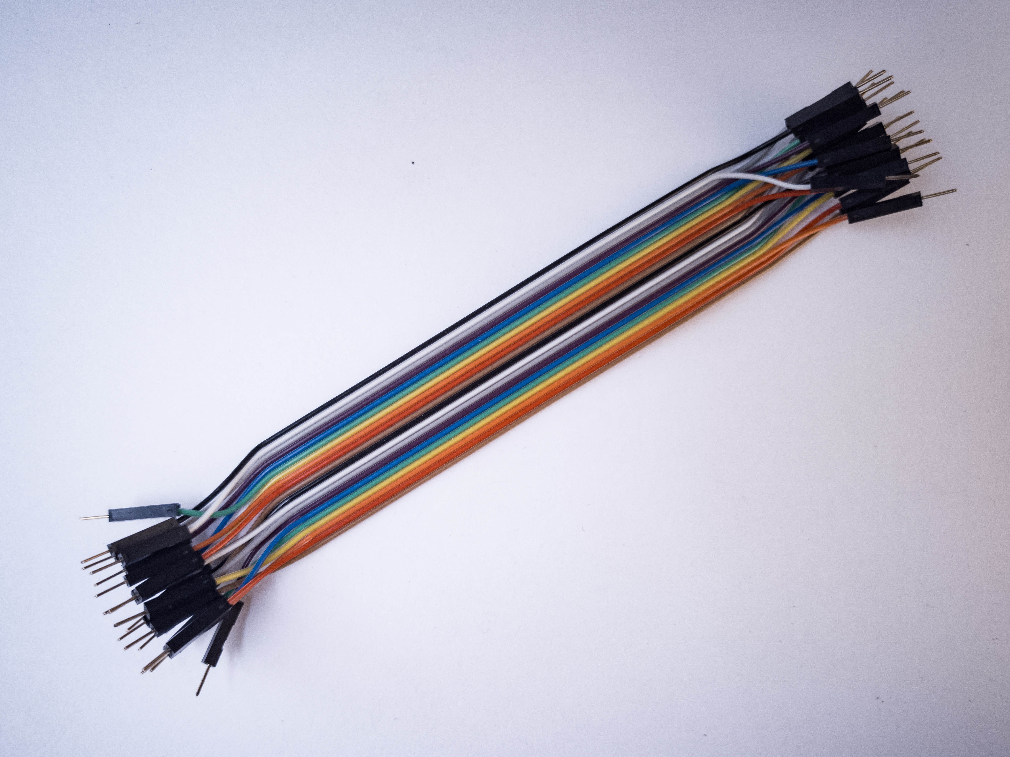
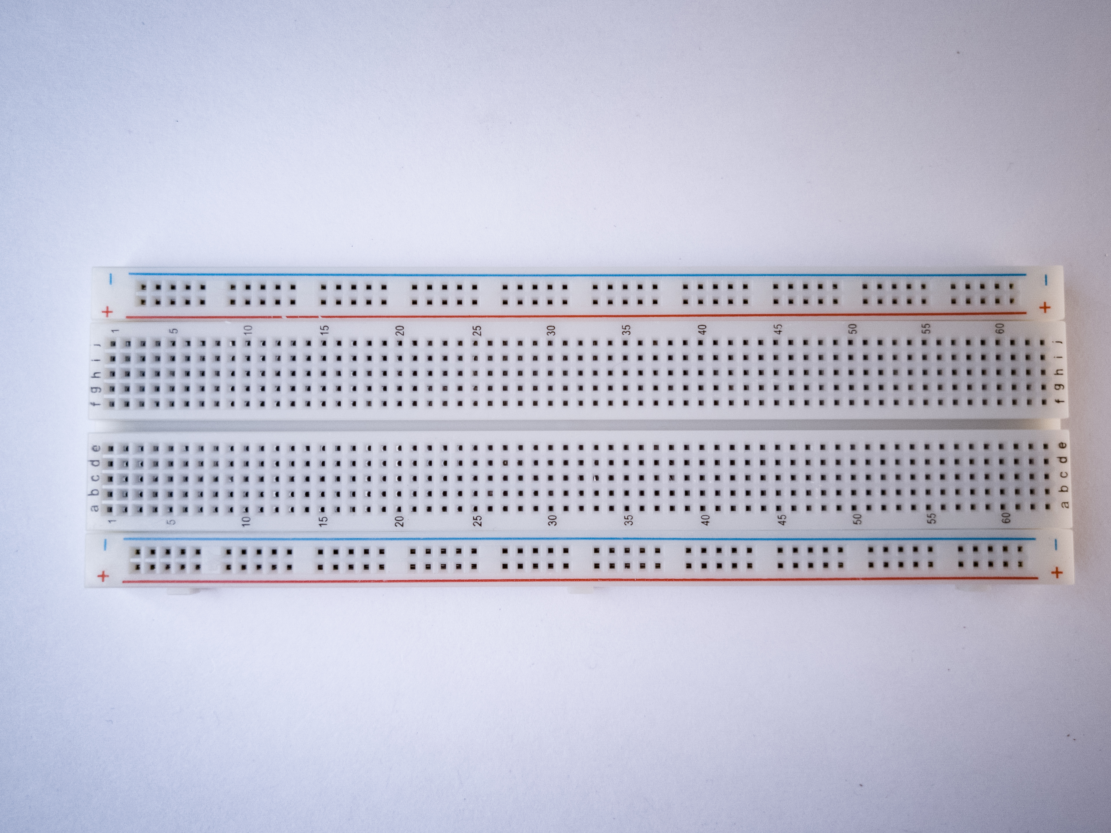
For this tutorial, gather the following components (see Figures 1–6 for reference images):
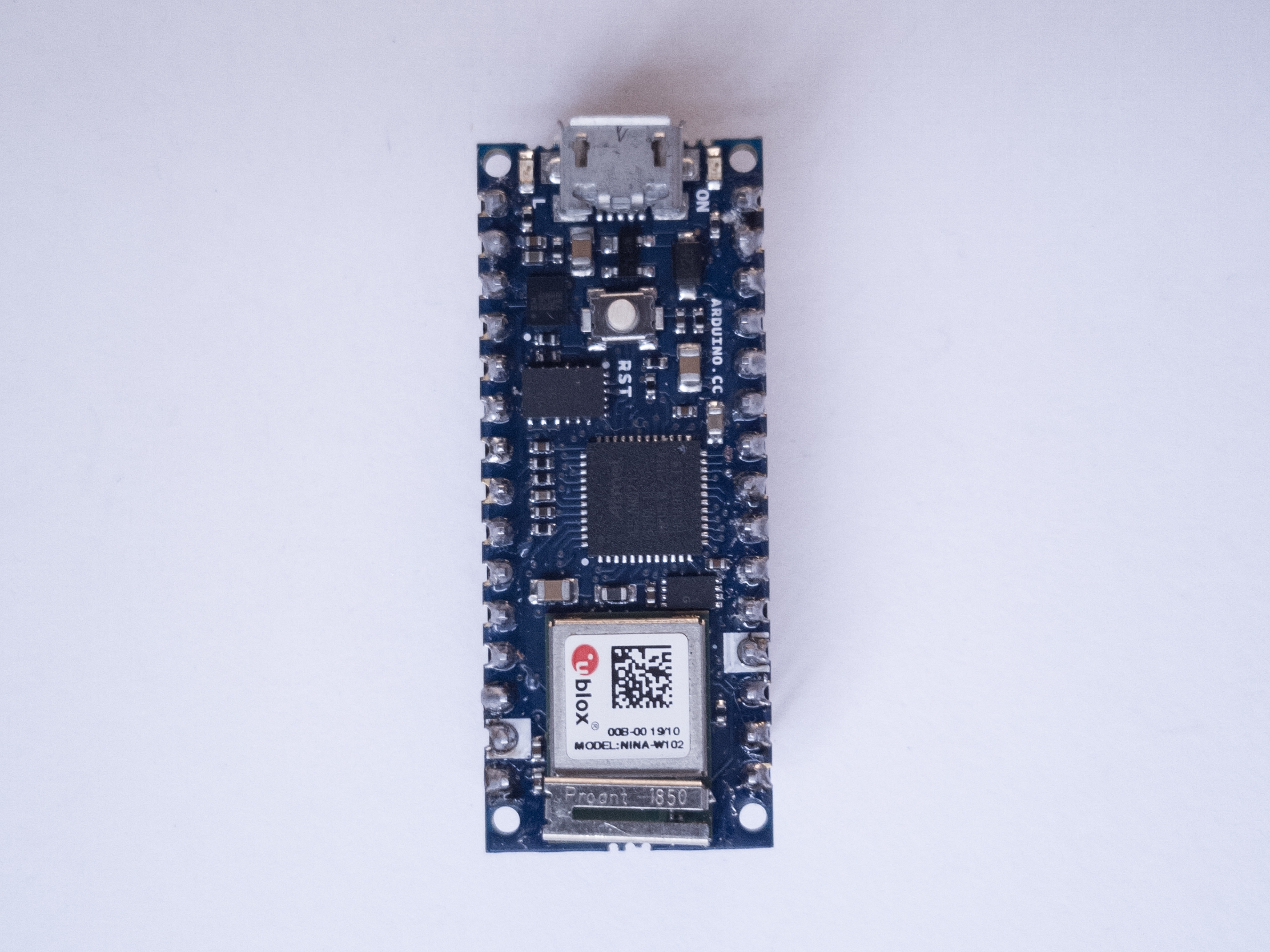
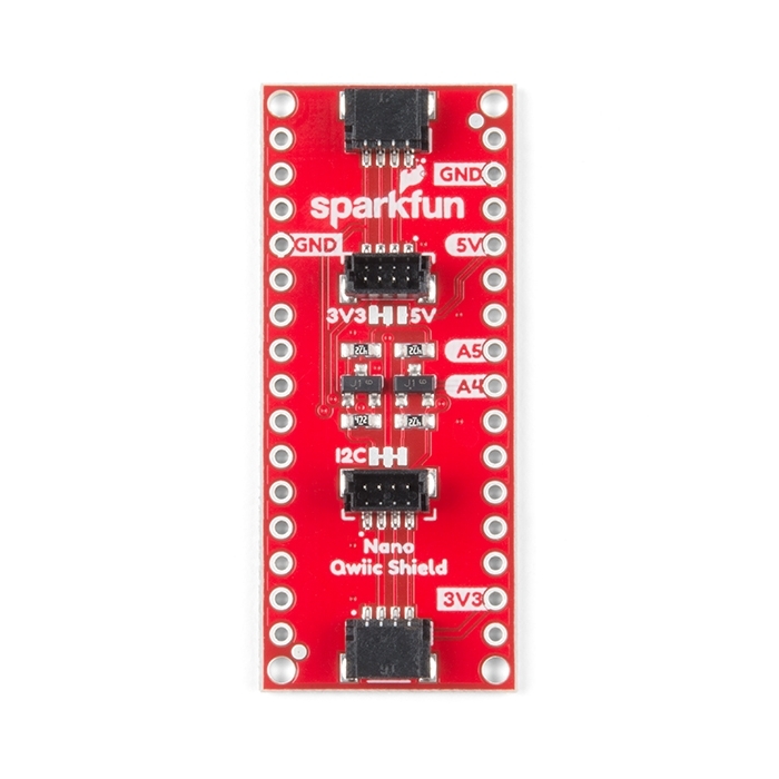
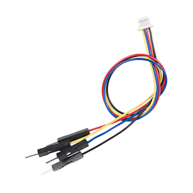
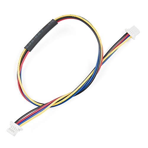
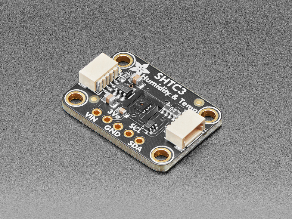
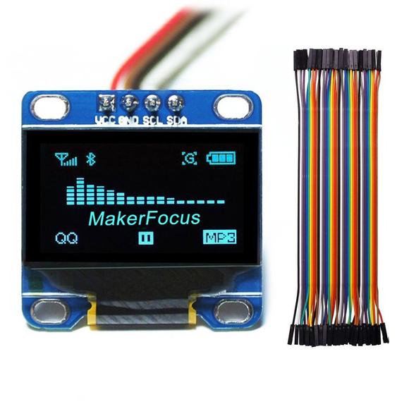
Figure 1. Arduino Nano 33 IoT or other Arduino Nano BoardFigure 2. SparkFun Qwiic Shield for Arduino NanoFigure 3. Qwiic Jumper Adapter CableFigure 4. Qwiic CableFigure 5. SHTC3 Temperature Humidity SensorFigure 6. I2C OLED Display Module 0.96 inches
Shield Orientation and Setup
Physical Orientation
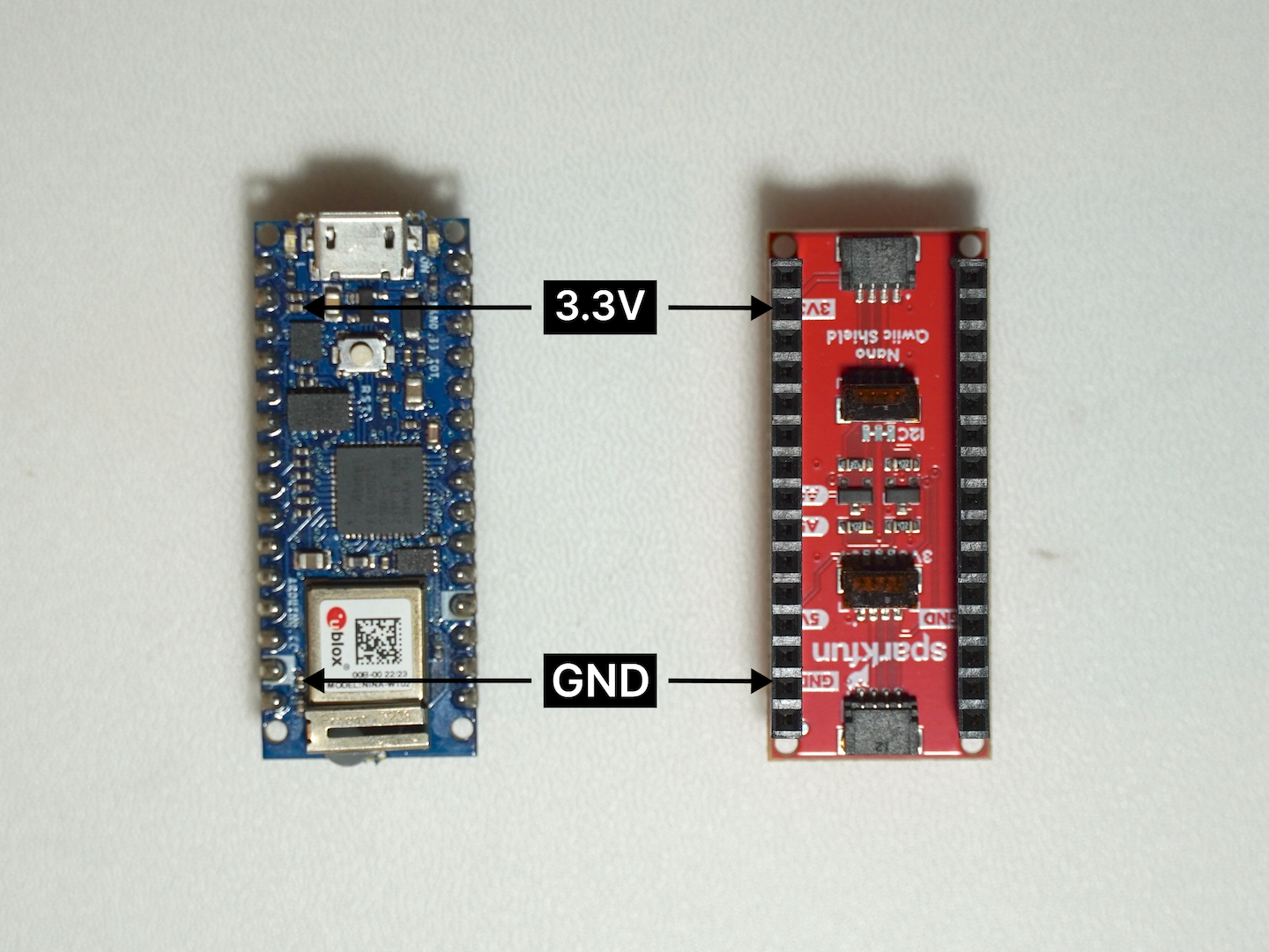
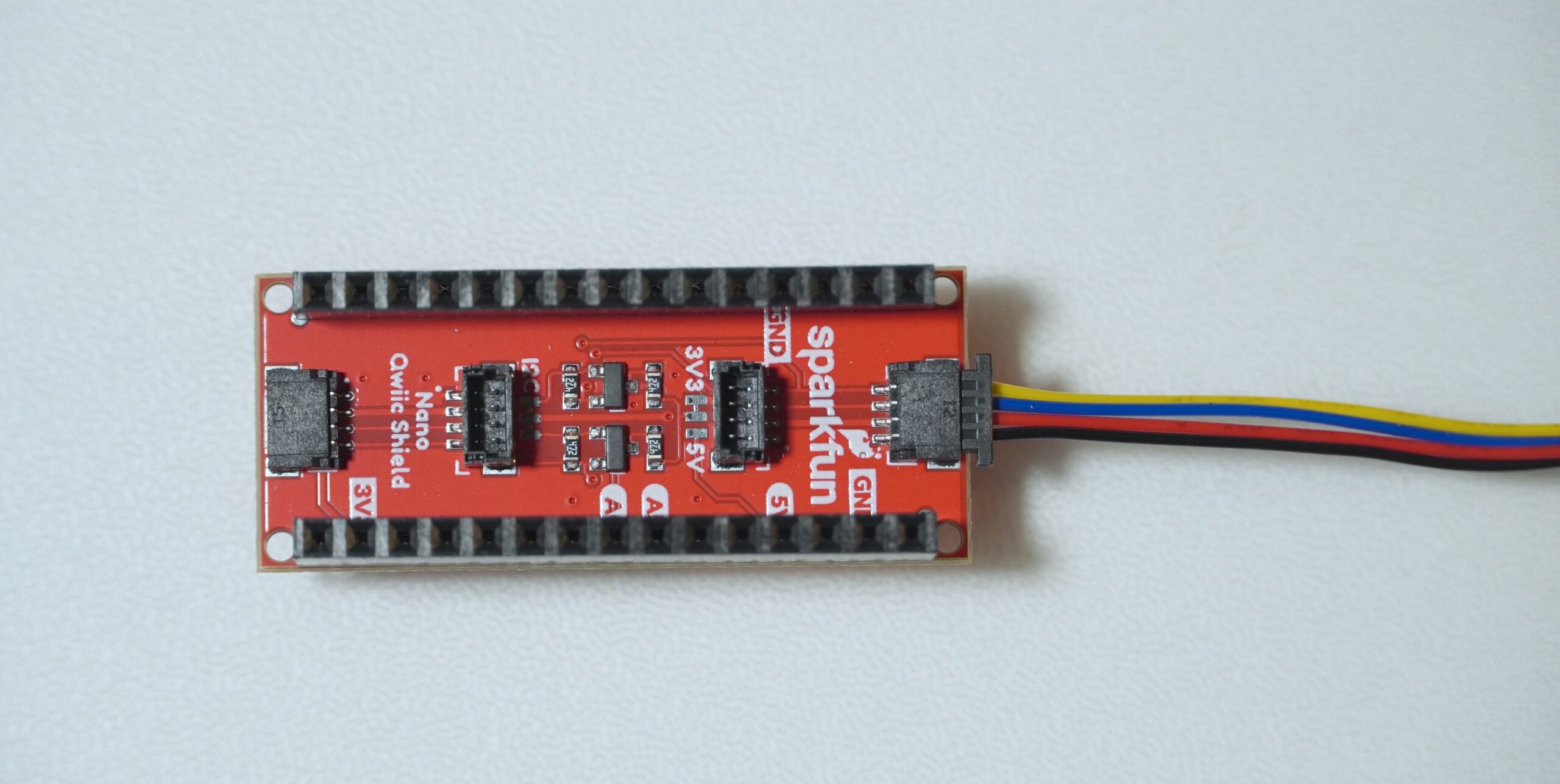
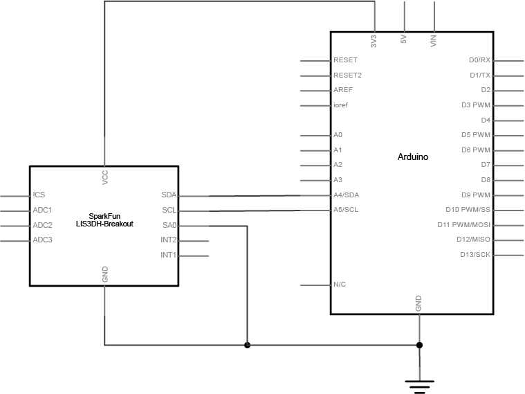
Although the SparkFun Qwiic Shield for Arduino Nano is pinned out exactly like a standard Arduino Nano, it’s still important to verify that you have the correct orientation when mounting the shield. We often reference the 3.3V pin as a quick visual cue to ensure you align everything properly. The shield includes a configurable logic shifting circuit set by the IOREF jumper, which defaults to 3.3V (ideal for boards like the Arduino Nano 33 BLE). If you’re using a 5V Nano variant (such as the Arduino Nano Every), you’ll need to switch the jumper to 5V so that the logic levels match your board’s operating voltage.
Figure 7. Pin alignment guide for powering the SparkFun Qwiic Shield using the Arduino Nano 33 IoT. Ensure that the GND and 3.3V pins are correctly connected to provide stable power and enable Qwiic-based I2C communication.
The Qwiic shield is designed to be mounted below the Nano with which it’s paired. To mount it below would require reversing the standard pin arrangement on the Nano (they are usually on the side of the board without components) and reversing the sockets on the shield.
Figure 8. Arduino on top of the Qwiic shield
Closer Look at the Adapter
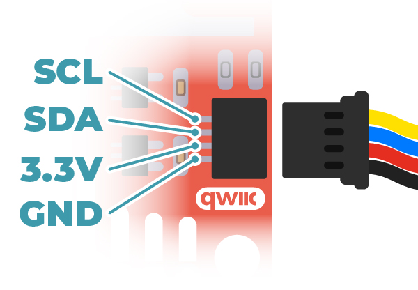
The Qwiic adapter is populated with two 4-pin 1mm JST connectors. These connectors are polarized to prevent incorrect insertion, and the pin order follows the Qwiic standard: GND, 3.3V, SDA, and SCL. When mounting the adapter onto the Nano Qwiic Shield, ensure that the labeled side of the adapter aligns with the corresponding pins on the shield to maintain correct orientation.
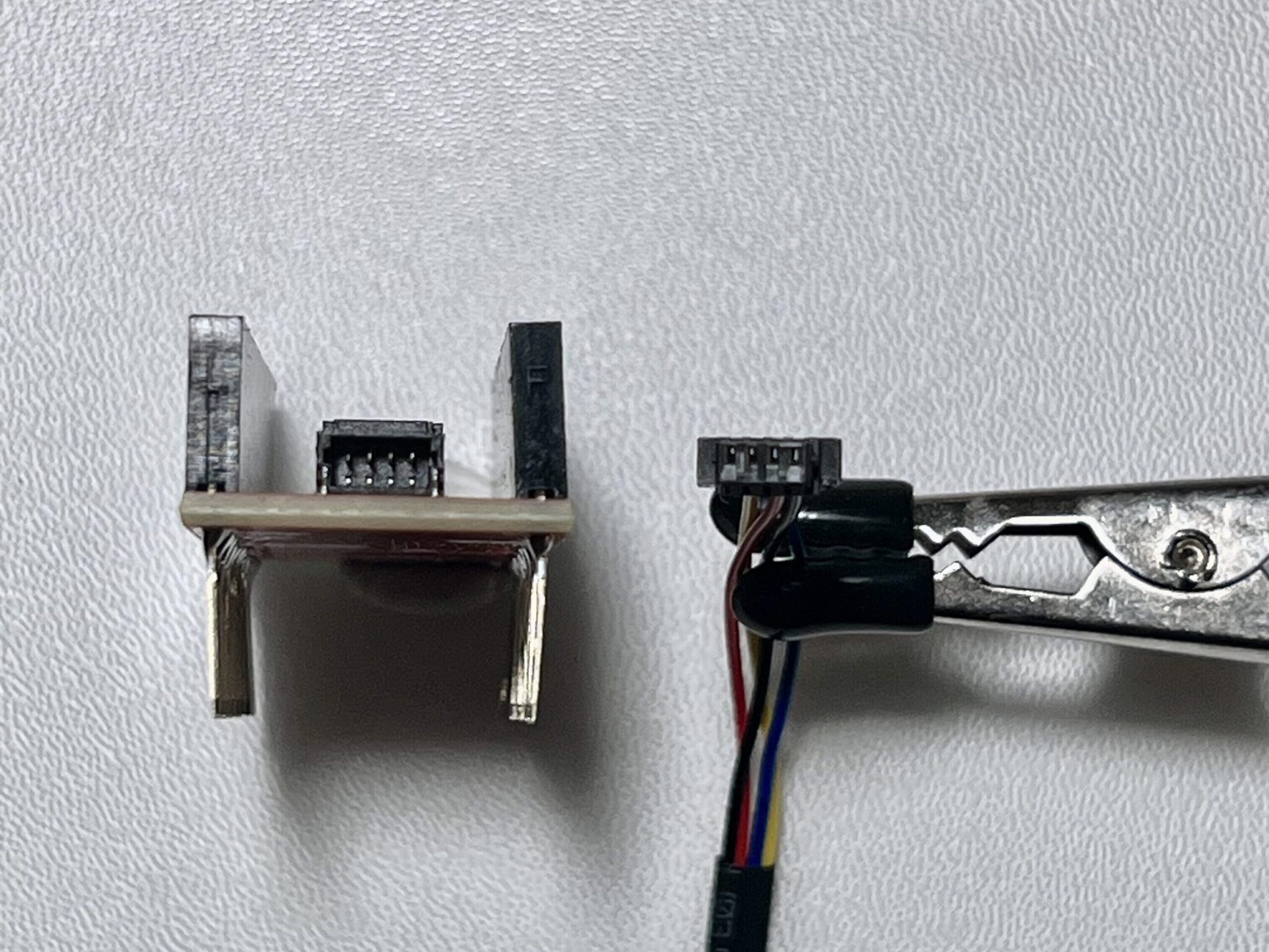
Figure 9. Qwiic connector pinout diagram showing the standard I2C wire order: SCL, SDA, 3.3V, and GND. The polarized JST connector ensures correct orientation, enabling plug-and-play communication between Qwiic-compatible devices without soldering. sourceFigure 10. A SparkFun Nano Qwiic Shield with a Qwiic cable connected, showing the standard I2C wire orientation. Figure 11. Connector alignment for Qwiic interface: the 4-pin JST cable is shown in correct orientation for insertion into the Qwiic Shield’s port
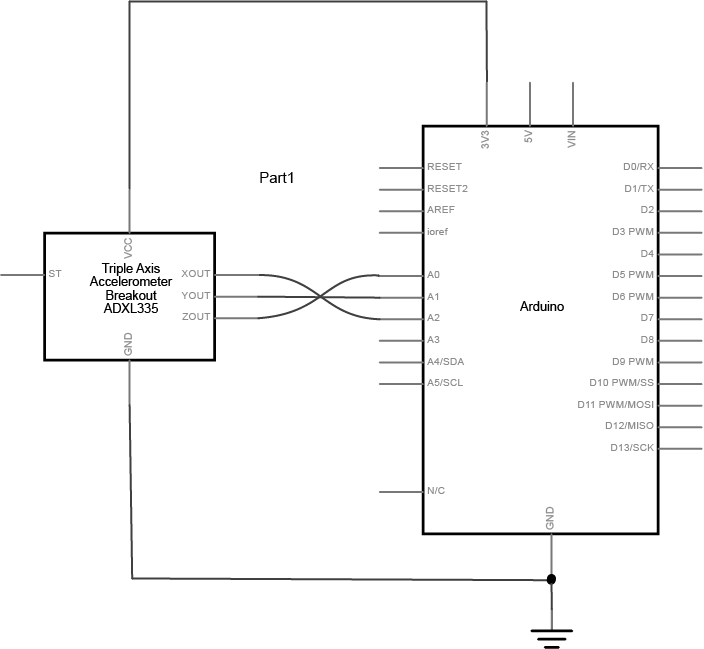
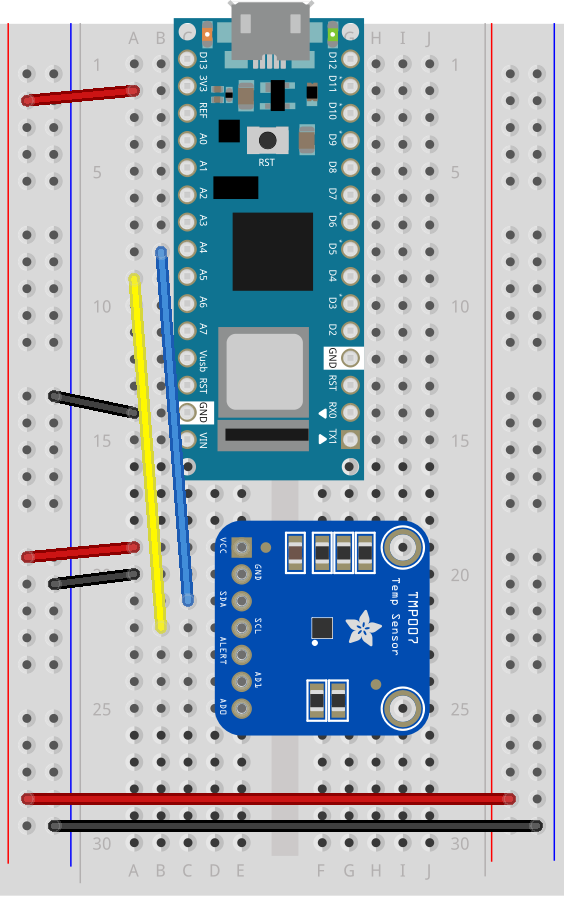
Connection Diagram
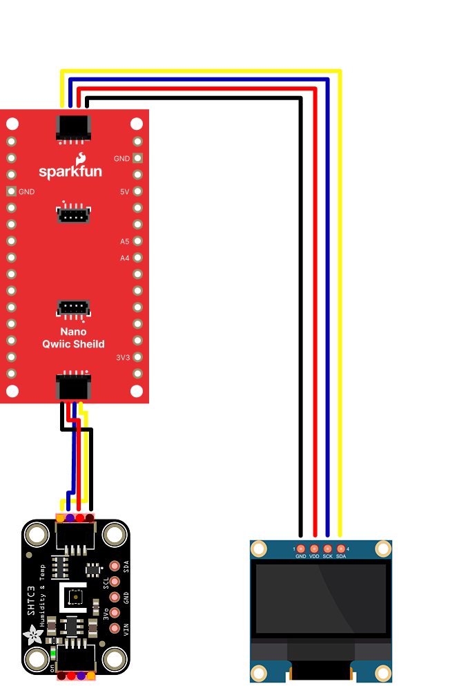
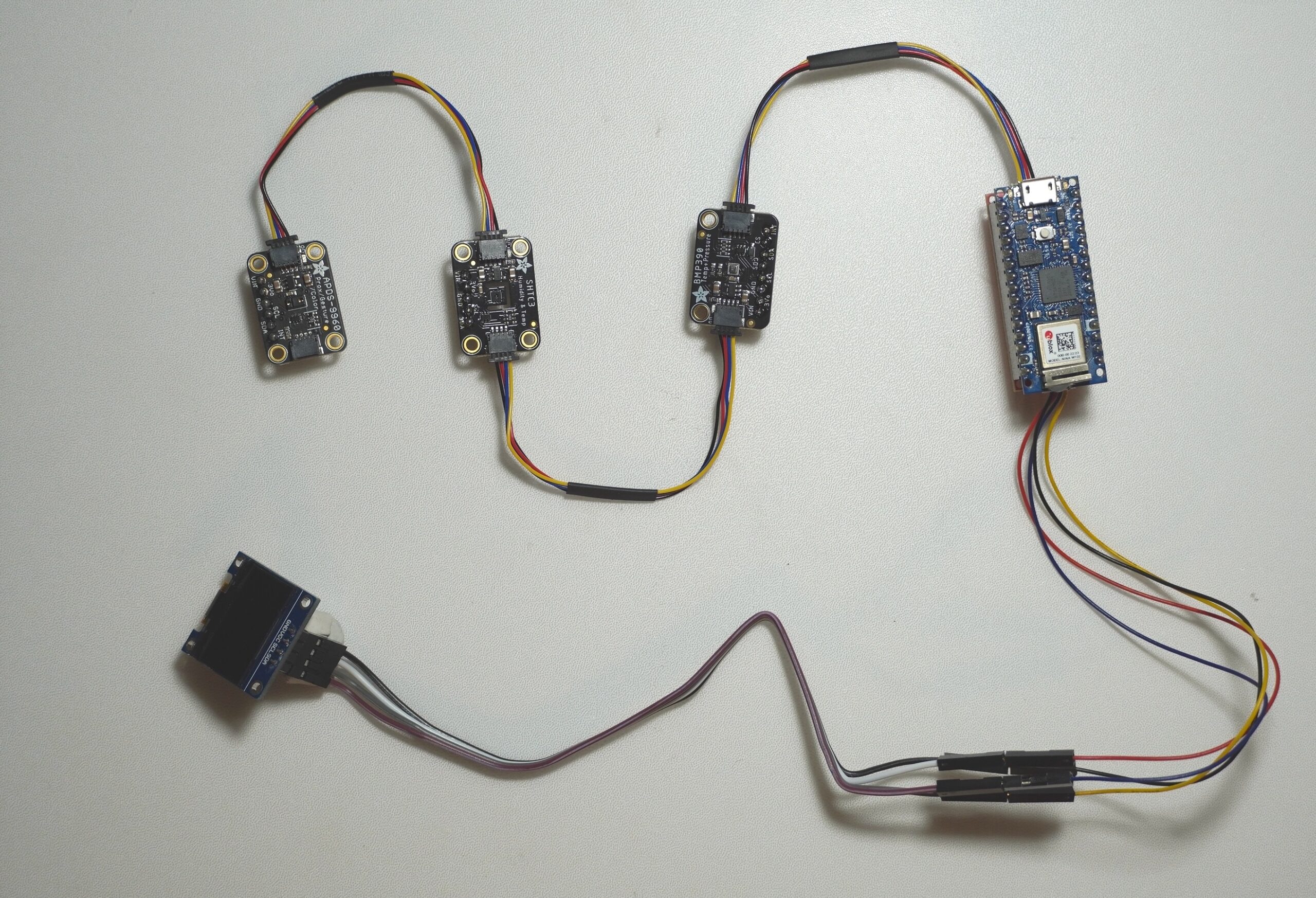
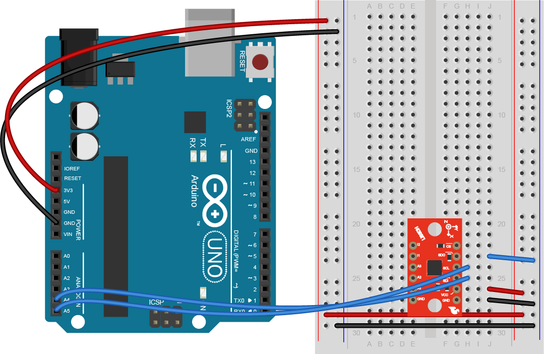
Figure 12 shows the connections between the Qwiic Nano shield and a few typical components.
Figure 12. Wiring diagram for a basic Qwiic I2C setup (Arduino below the shield is not shown in this diagram)
Note that while the Arduino Nano is not shown here, it is connected directly on top of the shield. Note also the placement of I2C communication pins (SDA and SCL). Ensuring the correct physical orientation prevents damage and guarantees reliable operation.
I2C Communication Overview
The SparkFun Qwiic Shield leverages the I2C protocol—a standard for connecting multiple devices with just two wires (SDA and SCL). This tutorial assumes that you’ve reviewed the ITP I2C Communication Labs or Related videos: Intro to Synchronous Serial, I2C for background on the protocol.
I2C Basics
Two-Wire Protocol: Communication occurs over SDA (data) and SCL (clock) lines.
Device Addressing: Each device on the I2C bus is identified by a unique 7-bit address.
Pull-up Resistors: These ensure proper voltage levels on the bus and are often integrated on breakout boards.
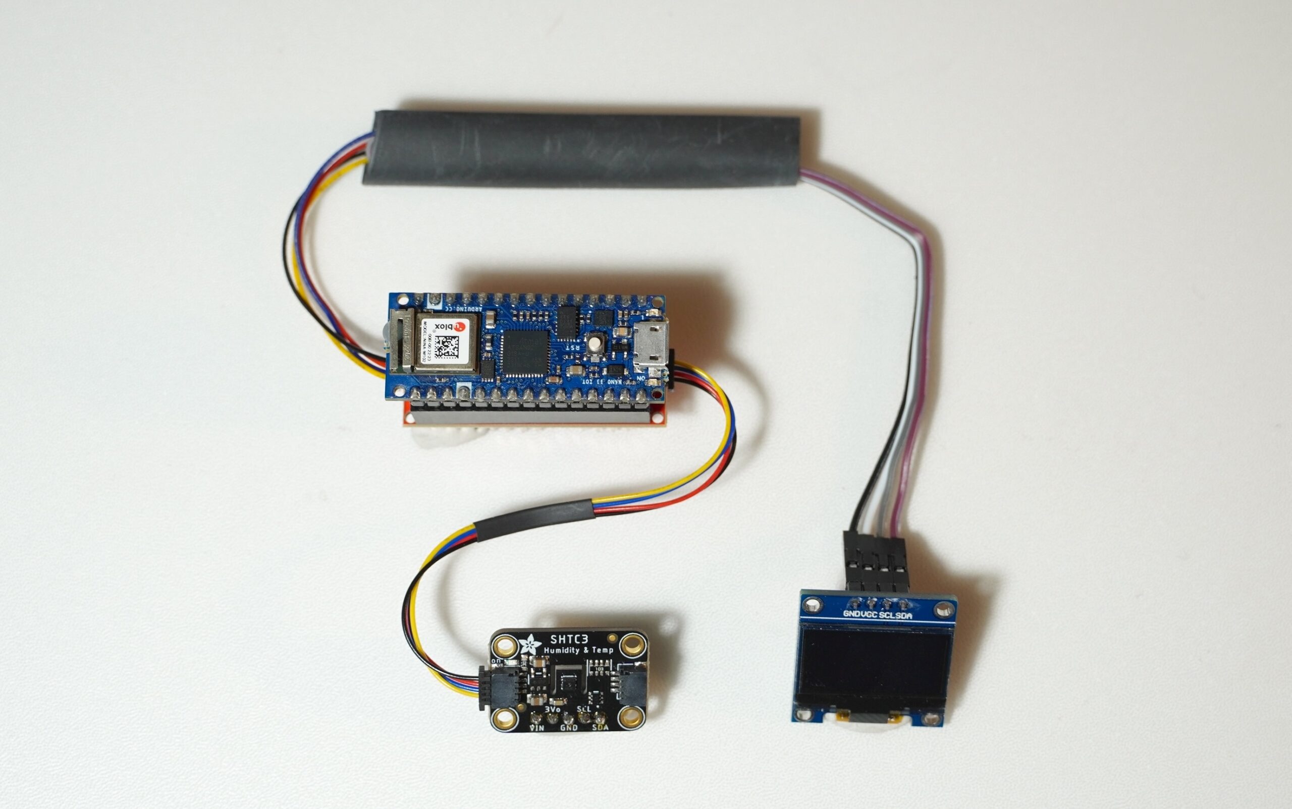
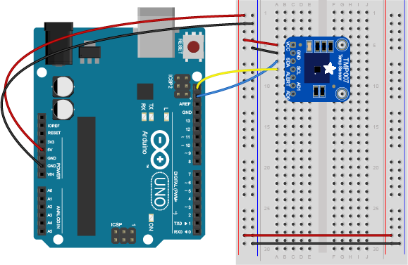
Demo Project: Reading Temperature and Humidity on an OLED Display
In this project, we’ll read data from SHTC3 (Humidity and Temp Sensor) and display it on an SSD1306 OLED screen. All components communicate via I2C and connect using Qwiic cables—no breadboards or soldering are required.
⚠️ Note: Many I2C sensors from providers like SparkFun (Qwiic) and Adafruit (STEMMA QT) come in two variants:
Qwiic/STEMMA QT-compatible versions, which feature JST connectors for plug-and-play wiring (see Figure 13 below) or
Standard breakout boards, which expose I2C pins (SDA, SCL, VCC, GND) but require jumper wires or soldering (see Figure 13 below)
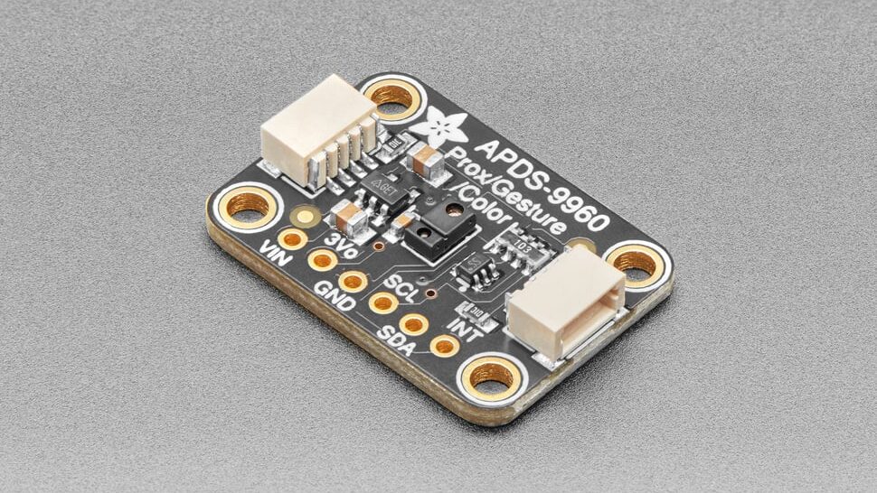
Figure 13. Adafruit APDS9960 Proximity, Light, RGB, and Gesture Sensor – with STEMMA QT / Qwiic connector source
For this demo, we’re using the Qwiic-compatible versions, enabling quick, tool-free connections. However, you can also use standard versions of the same sensors as long as you connect them properly to the corresponding I2C pins.
Hardware Setup
Mount the Shield
Carefully align the Arduino Nano 33 IoT (or other Nano variant) with the SparkFun Qwiic Shield for Arduino Nano.
Ensure the 3.3V pins line up correctly to avoid damaging your board.
Connect the Sensors
Connect sensors to any available Qwiic port using Qwiic cables.
Daisy-chain sensors as needed for project layout.
Attach the OLED Display
If the OLED display includes a Qwiic connector, directly connect it to a free port or daisy-chain.
If not, use a Qwiic Jumper Adapter Cable to connect the necessary pins.
Power and Ground
The Nano’s USB port powers the setup, with the Qwiic Shield distributing 3.3V and GND.
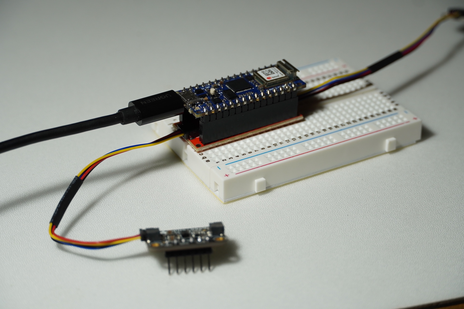
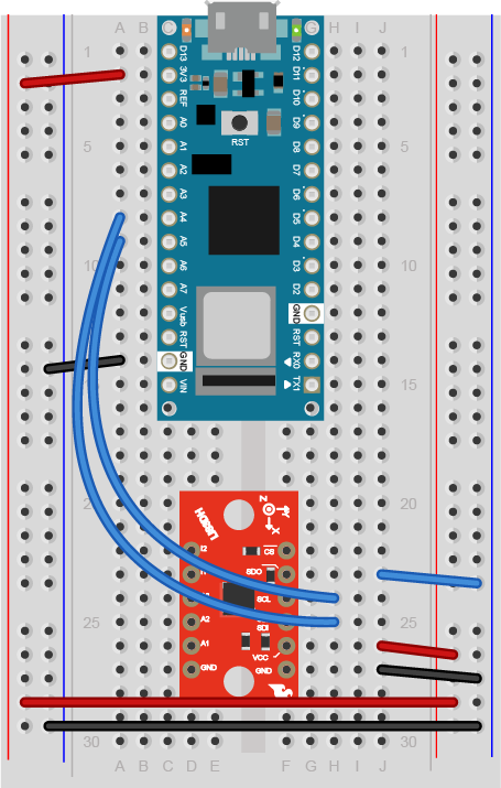
Figure 15. A compact I2C sensor-to-display demo using the Arduino Nano 33 IoT and SparkFun Qwiic Shield.
Install the External Libraries
In the Arduino IDE’s Library Manager (Sketch > Include Library > Manage Libraries…), install the following libraries and dependencies if needed.
In the demo code below, we begin by importing the necessary libraries and defining display parameters such as screen size and I2C address. In the setup() function, we initialize both the SHTC3 sensor and the OLED display, and configure display settings including text size, font, and color. In the loop(), the code reads humidity and temperature data from the sensor every three seconds and updates the OLED screen to show the latest values.
// Libraries for sensor and display communication
#include <SPI.h>
#include <Wire.h>
#include <Adafruit_GFX.h>
#include <Adafruit_SSD1306.h>
#include <Adafruit_SHTC3.h>

// Instantiate sensor object
Adafruit_SHTC3 shtc3 = Adafruit_SHTC3();

// OLED display resolution and initialization
#define SCREEN_WIDTH 128
#define SCREEN_HEIGHT 64
#define OLED_RESET -1 // because the reset pin on the OLED is not being used
#define SCREEN_ADDRESS 0x3C
Adafruit_SSD1306 display(SCREEN_WIDTH, SCREEN_HEIGHT, &Wire, OLED_RESET);

void setup() {
  // initialize serial communication
  Serial.begin(9600);
  // wait 3 seconds if the serial monitor is not open:
  if (!Serial) delay(3000);

  // Initialize SHTC3 sensor, loop indefinitely if this fails:
  if (!shtc3.begin()) {
    Serial.println("Couldn't find SHTC3");
    // stop forever if the sensor is not available:
    while (true);
  }
  Serial.println("Found SHTC3 sensor");

  // Initialize OLED display, halt program if allocation fails
  if (!display.begin(SSD1306_SWITCHCAPVCC, SCREEN_ADDRESS)) {
    Serial.println(F("Couldn't find SSD1306 screen"));
    // stop forever if the display fails:
    while (true);
  }

  // Configure display settings
  display.setTextSize(1);
  display.setTextColor(SSD1306_WHITE);
  display.cp437(true);
}

void loop() {
  // make instances of the sensor elements from the sensor library:
  sensors_event_t humidity, temp;

  // Get fresh data from sensor
  shtc3.getEvent(&humidity, &temp);

  // Clear OLED display and set cursor to start
  display.clearDisplay();
  display.setCursor(0, 0);

  // Display temperature readings
  display.println("Temperature: ");
  display.print(temp.temperature);
  display.println(" °C");
  display.println("");

  // Display humidity readings
  display.println("Humidity: ");
  display.print(humidity.relative_humidity);
  display.println("% rH");

  // Update display with new data
  display.display();

  // Wait for 3 seconds before refreshing
  delay(3000);
}
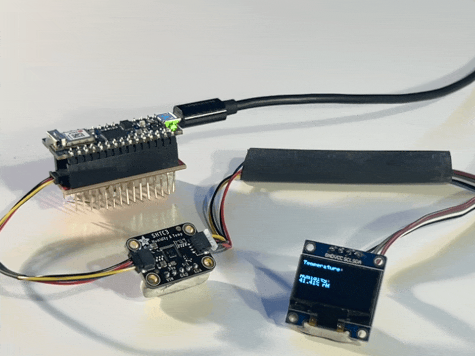
Final Result
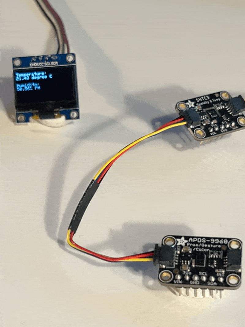
Figure 16. Real-time environmental monitoring demo using an Arduino Nano with SparkFun’s Qwiic Shield. The SHTC3 sensor measures temperature and humidity, displaying live data on the SSD1306 OLED screen
Further Use Cases
For a more advanced setup, we can expand the I2C chain by adding more sensors or devices. In the demo below, there is an APDS-9960 gesture sensor and a BMP388 pressure sensor alongside the SHTC3 temperature and humidity sensor. The user can change the data display on the screen by simple hand movement. You can find examples for these sensors at this link.
Figure 17. Chain of I2C sensors and display connected to an Arduino Nano 33 IoT using SparkFun’s Qwiic system.Figure 18. Live sensor data in action—temperature and humidity readings from an SHTC3 sensor are displayed on an OLED screen, while an APDS-9960 gesture and proximity sensor is also daisy-chained via Qwiic. This setup demonstrates how multiple I2C devices can work together seamlessly over a single bus.
Conclusion
The Sparkfun Qwiic Shield can simplify sensor integration and communication with Arduino Nano variants. It’s not the only way to connect IC components, but if you are, and if you’re using a Nano, it’s a handy tool. Whether you’re building a simple temperature monitor or a more complex interactive installation, understanding the practicalities of shield orientation, I2C communication, and connection strategies is key.
In this lab, you’ll see synchronous serial communication in action using the Inter-integrated Circuit (I2C) protocol with a time-of-flight distance sensor and a microcontroller.
Many different sensors on the market use the I2C protocol to communicate with microcontrollers. It is the most common way to connect to advanced sensors these days. The VL53L0X used in this lab is typical of an I2C sensor, so the principles covered here will help you when working with other I2C sensors as well. Much of this lab is adapted from the I2C lab on the APDS-9960 Color, Light, and Gesture Sensor.
Figure 1-3 are the parts that you need for this lab.
Figure 1. 22AWG solid core hookup wires.
Figure 2. Arduino Nano 33 IoT or other Arduino board
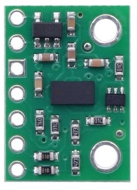
Figure 3. A VL53L0X distance sensor breakout board.
Sensor Characteristics
The sensor used in this lab, an ST Micro VL53L0X sensor, is an integrated circuit (IC) that can read the distance out to about 2000mm. It uses a 940 nm VCSEL emitter (Vertical Cavity Surface-Emitting Laser) that reflects off the target to determine the distance. There are breakout boards available for this sensor from multiple vendors, including Adafruit and Pololu (all available through Digikey, among others) .
I2C Connections
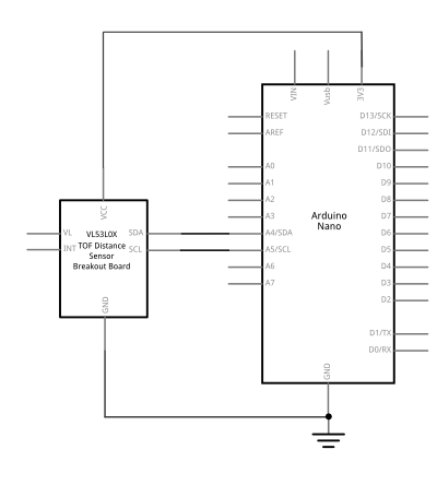
Connect the sensor’s voltage and ground pins to your voltage and ground buses, and the I2C clock (SCL) and I2C serial data (SDA) pins to your microcontroller’s corresponding I2C pins as shown in Figure 4-6. The schematic, Figure 4, is the same for both the Uno and the Nano. For the Arduino Uno or the Arduino Nano boards, the I2C pins are pins A4 (SDA) and A5(SCL). This is the same connection for almost any I2C sensor.
Some I2C sensors also have a few other pins:
an interrupt pin, used to signal the microprocessor when a reading is ready.
a shutdown or reset pin, used for powering down or resetting the sensor.
For this exercise, you won’t be using interrupt or shutdown pins.
What are Qwiic/Stemma/Grove/Gravity?
In addition to the standard I2C connections, Sparkfun and Adafruit use a connector called Qwiic which connects the I2C, power, and interrupt connectors all in one cable, eliminating the need for soldering. It’s a Sparkfun brand name. However, you’ll need a Qwiic adapter shield to use it. Adafruit have a similar brand called Stemma, Seedstudio uses Grove, and DFRobot uses Gravity. They all support I2C and have custom solderless connectors, though their connectors are not compatible with each other. To maintain compatibility, stick with the I2C header pins.
Figure 4. Schematic view of an Arduino attached to an VL53L0X sensor. This is the typical schematic for most I2C sensors.
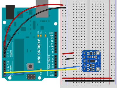
Figure 5. Breadboard view of an Arduino attached to a VL53L0X sensor. This shows an Adafruit breakout board, but other companies’ boards use the same pins: voltage, ground, SDA, and SCL.
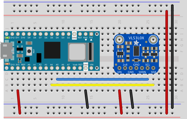
Figure 6. A VL53L0X distance sensor breakout board connected to an Arduino Nano 33 IoT. This shows an Adafruit breakout board, but other companies’ boards use the same pins: voltage, ground, SDA, and SCL.
The circuit is now complete, and you’re ready to write a program to control it. One of the advantages of the I2C synchronous serial protocol (as opposed to the SPI protocol) is that you only ever need two wires for communication to one or multiple devices.
How I2C Sensors Work
I2C devices exchange bits of data whenever the shared clock signal changes. Controller and peripheral devices both send bits of data when the clock changes from low to high (called the rising edge of the clock). Unlike with SPI, they cannot send data at the same time.
The Vl53L0X has a series of memory registers that control its function. You can write to or read from these registers using I2C communication from your microcontroller. Some of these registers are writable by the controller so that you can configure the sensor. Some registers are configuration registers. Writing to them sets the sensor’s characteristics. For example, you can configure whether the sensor is in high speed mode, high sensitivity mode, or long distance mode. Other memory registers are read-only. For example, when the sensor has read the proximity of an object, it will store the result in a register that you can read from the controller. The details of the chip’s registers can be found in thesensor’s datasheet.
How I2C Bits are Exchanged
Most of the time, you never have to think about how the bits of an I2C message are exchanged. If so, then you might want to skip to the the next section on I2C Libraries. For the low-level details, read on:
I2C devices exchange data in 7-bit chunks, using an eighth bit to signal if you’re reading or writing by the controller or for acknowledgement of data received. The top seven bits of a byte are the data bits, and the bottom bit is the read/write bit. To get the distance from the VL53L0X, your controller device sends the sensor’s address (a 7-bit number, for this sensor it’s 0×29) followed by a single bit indicating whether you want to read data or write data (1 for read, 0 for write). That means the address byte is 0x53 for read, 0x52 for write access. Then you send the memory register in which the sensor’s ranging data is stored. The sensor then sends the value of that register back to you. For this particular sensor, STMicro wraps the control register documentation in an abstracted API, described in this document. The section labeled “Define Registers” lists all the registers and their addresses. The RESULT_RANGE_STATUS register is the register that holds the latest distance reading.
I2C and the Wire Library
The Wire library, which is built into the Arduino IDE, is the main library for accessing I2C communication. However, most Arduino-compatible I2C device libraries incorporate this library, but don’t expose it directly in their APIs. This makes things simpler for the user. Instead of having to work out the details described above, for example, you can just call a function like readRangeResult() which does the I2C work for you.
The libraries for this sensor are typical of this style of library. For example, the Adafruit_VL53L0X library’s startRange() command sends a write command to start a reading of the sensor. The isRangeComplete() sends a read command to read the register that indicates whether or not the reading is done.
All sensors take a certain amount of time to read the physical phenomena which they sense. With light-based sensors like the VL53L0X, the time they take to get a reading is usually called ranging time, or ranging measurement time, and it’s noted in the data sheet how long it is (about 23ms). In operation, you query the sensor as to whether it’s got a reading available, and then read it when that’s true.
How To Pick a Library
Most companies that make breakout boards for a given I2C sensor will also write a library for it. A search on the term “VL53L0X” in the Arduino library manager will return several libraries. All of them will work with any of the breakout boards. What’s the difference? Ideally, you want a library that works well, has readable examples, and good documentation. Often you have to settle for two of the three.
Different companies and programmers have different styles for writing a library’s application programming interface, or API. Arduino has a style guide for writing APIs, but it’s not always followed by others. The Arduino-developed libraries generally follow this guide. Other companies’ libraries may have a few more configuration functions, and their examples are a bit more complicated as a result. You should look at the examples with any library to see if they make sense to you. A good guideline is to use the library with the instructions and examples that you find to be the clearest. Here is the Adafruit guide for this sensor. As you can see, it doesn’t tell you much about the functions themselves. However, you can also get information from the library’s header file. The header file is generally the file with the name libraryname.h. Sometimes it’s in a directory called src. For example, here’s the header file for the Adafruit_VL53L0X library. Within the header file, there are class names for the library and a section called public where you’ll find all the possible function definitions.
Even if the examples don’t include all the functions, the public section of the header file will. From there, you can build your own examples if the library’s examples don’t show how to use a function you want to use.
Adafruit’s library for this sensor is quite complex, and includes two different ways of reading the sensor. In their examples, they use a function called rangingTest(), which puts data into an object in memory called measure in the examples, and then you pull the readings from that object. However, you can also read the results directly using a set of simpler functions:
startRange() – starts the sensor taking a single reading
readRange() – returns a single range reading
readRangeResult() – returns a single range reading, and an error value (oxFFFF) if there’s an error
startRangeContinuous() – starts the sensor reading continuously
isRangeComplete() – returns true when a reading is complete and ready to be read
waitRangeComplete() – does nothing until the reading is complete
Pololu’s library is similar, but the API is a bit simpler, and their header file lists all the register addresses, for those interested in the lower-level details. They document all the functions on their repository’s main page as well. Their product documentation is clear, if shorter than Adafruit’s.
Install the External Libraries
You can use the library manager to find these libraries. Make sure you’re using Arduino version 1.8.14 or later. From the Sketch menu, choose Include Library, then Manage Libraries, and search for VL53L0X. All of the related libraries mentioned here will show up. The examples below use the Adafruit_Vl53L0X library.
Program the Microcontroller
At the beginning of your code, include the appropriate libraries. In the setup(), initialize the sensor with a function called begin() (Sparkfun sometimes uses init() instead of begin()). If the sensor responds, then begin() will return true; if not, it will return false. This is how to check that the sensor is properly wired to your microcontroller, and to configure it:
// include library
#include "Adafruit_VL53L0X.h"

// make an instance of the library:
Adafruit_VL53L0X sensor = Adafruit_VL53L0X();

const int maxDistance  = 2000;

void setup() {
  // initialize serial, wait 3 seconds for
  // Serial Monitor to open:
  Serial.begin(9600);
  if (!Serial) delay(3000);

  // initialize sensor, stop if it fails:
  if (!sensor.begin()) {
    Serial.println("Sensor not responding. Check wiring.");
    while (true);
  }
  /* config can be:
    VL53L0X_SENSE_DEFAULT: about 500mm range
    VL53L0X_SENSE_LONG_RANGE: about 2000mm range
    VL53L0X_SENSE_HIGH_SPEED: about 500mm range
    VL53L0X_SENSE_HIGH_ACCURACY: about 400mm range, 1mm accuracy
  */
  sensor.configSensor(Adafruit_VL53L0X::VL53L0X_SENSE_LONG_RANGE);
  // set sensor to range continuously:
  sensor.startRangeContinuous();
}
In the main loop() function, you’ll read the sensors. You’re going to query the sensor to see if it’s got a reading available with the isRangeComplete() function, then you’ll use the readRangeResult() function to get the result. This function returns a result in millimeters:
void loop() {
  // if the reading is done:
  if (sensor.isRangeComplete()) {
    // read the result:
    int result = sensor.readRangeResult();
    // if it's with the max distance:
    if (result < maxDistance) {
      // print the result (distance in mm):
      Serial.println(result);

    }
  }
}
Run this sketch now, and it will print out the distance from the sensor in millimeters (link to the full sketch).
Conclusion
I2C is a common protocol among many ICs, and it’s handy because you can combine many devices on the same bus. When doing so, however, make sure the device addresses are unique. This can complicate things if you want to use multiple sensors of the same type on the same I2C bus. Fortunately, this is not often the case.
In this lab, you’ll learn how to use a rotary encoder as an input to a microcontroller.
Introduction
Rotary encoders are sensors which sense the rotation of a central shaft. Unlike a rotary potentiometer, encoders can turn infinitely, covering the full 360 degrees of the shaft’s rotation. Many have built-in pushbuttons as well. Encoders are often used to measure the rotation of a vehicle’s wheel or axle as well. In this lab, you’ll learn how to use a rotary encoder as an input to a microcontroller.
What You’ll Need to Know
To get the most out of this Lab, you should be familiar with the following concepts beforehand. If you’re not, review the links below:
Figures 1-4 show the parts you’ll need for this exercise. Click on any image for a larger view.
Figure 1. Microcontroller. Shown here is an Arduino Nano 33 IoT, but an Uno will work as well
Figure 2. Jumper wires. You can also use pre-cut solid-core jumper wires.
Figure 3. A solderless breadboard
Figure 4. A rotary encoder with built-in pushbutton.
How the Sensor operates
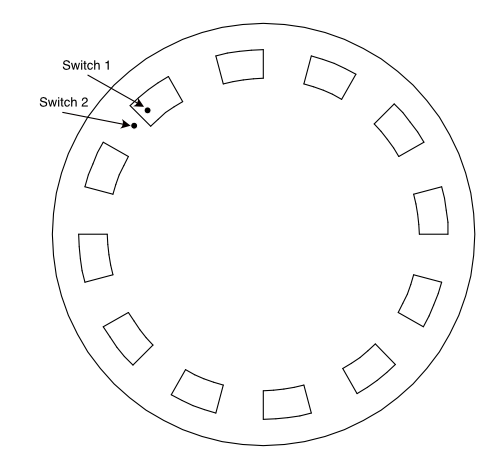
Rotary encoders measure rotation using two internal switches very close together, and a rotating disk. The disk has holes in it, and when the it passes each switch, the switch opens then closes. The switches open and close out of phase with each other, and the resulting pattern of open and close lets you detect the rotation. This is called quadrature encoding. Figure 5 shows a quadrature wheel and the positions of two switches relative to the wheel.
Figure 5. An encoder wheel. Several holes are spaced around the wheel near the edge. In this case, each hole has a 15-degree sweep, and is separated from the next hole by another 15 degrees. Two switches, separated by less than the sweep, are positioned so that the holes will pass them as the wheel turns.
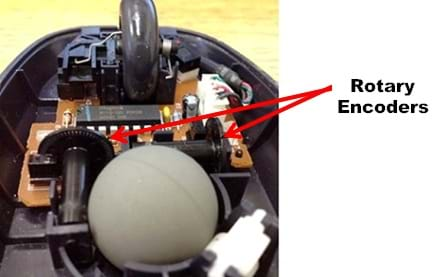
The sensors in an encoder may be mechanical or optical. Optical sensors (photodiodes) are often used to reduce mechanical wear on the sensor. Optical encoder wheels were common in early computer mice. You can see one in Figure 6, which comes from teachengineering.com
Figure 6. Inside a mechanical computer mouse. The wheel inside hangs out the bottom of the mouse. It rotates against the surface of your desk, turning two encoder wheels, one for the vertical direction and one for the horizontal.
An encoder doesn’t tell you its absolute position, but it does tell you whether it’s rotating left or right, depending on the pattern of the sensor changes. The amount of rotation, and therefore the resolution of the encoder, depends on how many holes the encoder has. The more holes, the more finely you can read the change in rotation.
Encoders are often used as knobs that can turn a full 360 degrees, but they are also used in other applications to sense a changing rotation. Wheel encoders and shaft encoders can be used to count revolutions of a vehicle’s axle, for example. In this lab you’ll see how to use a knob-style encoder.
The Circuit
To use an encoder, you connect its two switches to two digital input pins of your microcontroller and look for changes. Because they can happen very fast, it’s wise to use inputs which can be hardware interrupts, meaning that they can read change as soon as the pin changes, not just when you use the digitalRead() command.
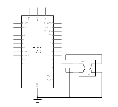
Figures 7 through 10 show how to connect an encoder with a pushbutton to an Arduino Nano 33 IoT or an Arduino Uno. For the Nano 33 IoT, any pin can act as a hardware interrupt pin. This lab uses pins 2 and 3 for compatibility with the Uno’s interrupts.
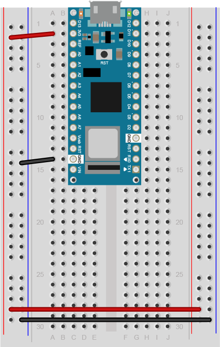
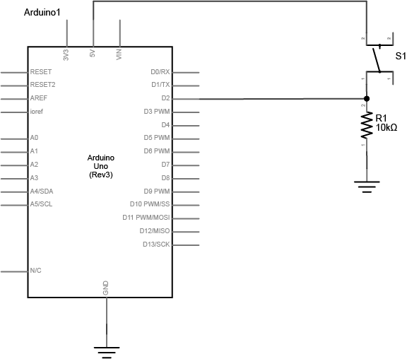
Figure 7. Schematic view of a rotary encoder with a pushbutton connected to an Arduino Nano 33 IoT. A typical encoder will have through-hole pins, with two pins on one side and three on the other. The side with three holes is the encoder, and the side with two holes is the pushbutton. The encoder’s two outer pins are attached to digital inputs 2 and 3. The encoder’s middle pin is attached to ground. One of the pushbutton’s two pins is attached to digital input 4. The other pin of the pushbutton is attached to ground.
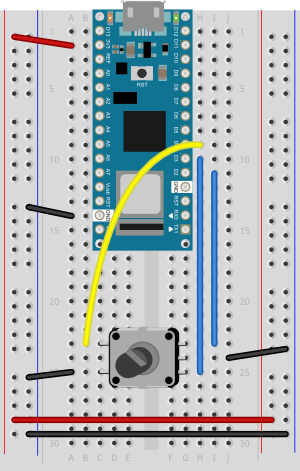
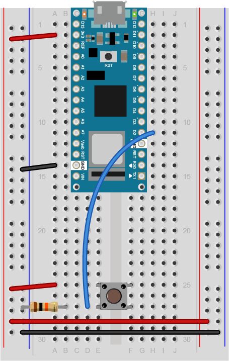
Figure 8. Breadboard view of a rotary encoder with a pushbutton connected to an Arduino Nano 33 IoT. This encoder and pushbutton is connected as described in Figure 7. The encoder’s two outer pins are attached to digital inputs 2 and 3. The encoder’s middle pin is attached to ground. One of the pushbutton’s two pins is attached to digital input 4. The other pin of the pushbutton is attached to ground.
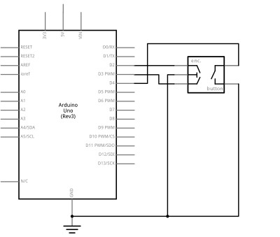
The wiring for an Arduino Uno is similar to the Nano 33 IoT, but the Nano has only two hardware interrupts, pins 2 and 3. It’s best to use those. If you are using a Nano 33 IoT, you can use any of that board’s interrupt pins if you wish instead. Those are pins 2, 3, 9, 10, 11, 13, A1, A5, and A7.
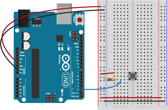
Figure 9. Schematic view of a rotary encoder with a pushbutton connected to an Arduino Uno. A typical encoder will have through-hole pins, with two pins on one side and three on the other. The side with three holes is the encoder, and the side with two holes is the pushbutton. The encoder’s two outer pins are attached to digital inputs 2 and 3. The encoder’s middle pin is attached to ground. One of the pushbutton’s two pins is attached to digital input 4. The other pin of the pushbutton is attached to ground.
Figure 10. Breadboard view of a rotary encoder with a pushbutton connected to an Arduino Uno. This encoder and pushbutton is connected as described in Figure 7. The encoder’s two outer pins are attached to digital inputs 2 and 3. The encoder’s middle pin is attached to ground. One of the pushbutton’s two pins is attached to digital input 4. The other pin of the pushbutton is attached to ground.
The Code
There are several libraries for reading interrupts. One of the earliest is Paul Stoffregen’s Encoder library referenced above, on which many others are based. That library doesn’t work with the Nano’s interrupts, however, so the examples below use Manuel Reimer’s EncoderStepCounter library instead.
To install it, search the Arduino IDE’s library manager for EncoderStepCounter by Manuel Reimer.
To read an encoder with the Encoder library, you include the library at the top, make an instance of the library in a variable in which you define the pins for the encoder. Then when you want to read the encoder, you call the .read() command. Here’s a basic example:
#include <EncoderStepCounter.h>

// encoder pins:
const int pin1 = 9;
const int pin2 = 10;
// Create encoder instance:
EncoderStepCounter encoder(pin1, pin2);

// encoder previous position:
int oldPosition = 0;

void setup() {
  Serial.begin(9600);
  // Initialize encoder
  encoder.begin();
}

void loop() {
  // if you're not using interrupts, you need this in the loop:
  encoder.tick();
  // read encoder position:
  int position = encoder.getPosition();

  // if there's been a change, print it:
  if (position != oldPosition) {
    Serial.println(position);
    oldPosition = position;
  }
}
When you run this, you’ll see that the position value goes up in one direction and down in the other. There is no absolute position; unlike a potentiometer, which measures an absolute resistance at a particular position of the wiper, an encoder reads only change in one direction or another. It doesn’t know where it is in the rotation, only how many steps it’s taken since it started counting steps.
Most knob-style encoders change with every click of the shaft. This is typical with many encoders. These clicks are called detents, and they are built into the shaft to give you a sense of its movement.
The EncoderStepCounter library will work on any digital pins of your board, but if you are not using interrupts, it may skip a step or two if you are turning the encoder fast. For this reason, it won’t work well for encoders that are not turned by a human hand, like the shaft encoders on many motors. You can correct for that by attaching it to interrupt pins, as described above. If you use interrupt pins, change your setup function as follows:
Then add a new function to handle the interrupts that will be generated:
// Call tick on every change interrupt
void interrupt() {
  encoder.tick();
}
If you enable interrupts like this, you won’t need the call to encoder.tick() in the loop() function.
When you run the sketch this time, you should see that the step value is changing once for each detent of the encoder shaft, and doesn’t miss steps.
If you want to make the step count reset itself when it reaches a maximum number of steps, you can do that by by changing the loop as shown below. This line resets the step counter every 24 steps by using the modulo, or remainder, operator (%):
void loop() {
  // if you're not using interrupts, you need this in the loop:
  encoder.tick();

  // read encoder position:
  int position = encoder.getPosition();

  if (position % 24 == 0) {
    encoder.reset();
    position = encoder.getPosition();
  }
  // if there's been a change, print it:
  if (position != oldPosition) {
    Serial.println(position);
    oldPosition = position;
  }
}
Rollover like this can be useful if you want the value to reset once per rotation.
The Pushbutton and Internal Pullup Resistors
Most knob-style encoders have a pushbutton built in as well, and you wired the encoder’s pushbutton in the diagram above. You may have noticed that it’s wired differently than you did in the digital in and out lab. There’s no pulldown resistor, and the pushbutton is wired to ground. What’s going on?
Many microcontrollers (including all Arduino models) have internal pullup resistors on the input pins. These function in the opposite way of a pulldown resistor: they pull the pin up to voltage when there’s no other connection. When you use an internal pullup resistor, you wire your pushbutton to ground instead of to voltage, and the pin goes low when you press the button. This saves you one resistor; all you have to do is to wire your pushbutton to ground from the digital input pin, and declare the pin’s mode like so: digitalWrite(buttonPin, INPUT_PULLUP); You’ll see it in the example below:
void setup() {
  // set the encoder's pushbutton to use internal pullup resistor:
  pinMode(4, INPUT_PULLUP);
  Serial.begin(9600);
}

void loop() {
  int buttonState = digitalRead(4);
  Serial.println(buttonState);
}
Upload this code to your board with the circuit as shown in figures 7 through 10, then open the serial monitor. Press the encoder push the encoder’s pushbutton to see how the state changes.
Putting It all Together
Using an encoder and its pushbutton together gives you a great way to let a user choose from a range of choices. By reading the changing encoder state, you can get the range, and by reading the pushbutton, you can get the one they chose. Here’s an example that reads both the encoder and the pushbutton to do just that:
#include <EncoderStepCounter.h>

const int pin1 = 2;
const int pin2 = 3;

// Create encoder instance:
EncoderStepCounter encoder(pin1, pin2);

// encoder previous position:
int oldPosition = 0;

const int buttonPin = 4;    // pushbutton pin
int lastButtonState = LOW;  // last button state
int debounceDelay = 5;      // debounce time for the button in ms


void setup() {
  Serial.begin(9600);
  // Initialize encoder
  encoder.begin();
  // Initialize interrupts
  attachInterrupt(digitalPinToInterrupt(pin1), interrupt, CHANGE);
  attachInterrupt(digitalPinToInterrupt(pin2), interrupt, CHANGE);
  // set the button pin as an input_pullup:
  pinMode(buttonPin, INPUT_PULLUP);
}

void loop() {
  // if you're not using interrupts, you need this in the loop:
  encoder.tick();

  // read encoder position:
  int position = encoder.getPosition();
  // read the pushbutton:
  int buttonState = digitalRead(buttonPin);
  //  // if the button has changed:
  if (buttonState != lastButtonState) {
    // debounce the button:
    delay(debounceDelay);
    // if button is pressed:
    if (buttonState == LOW) {
      Serial.print("you pressed on position: ");
      Serial.println(position);
    }
  }
  // save current button state for next time through the loop:
  lastButtonState = buttonState;

  // reset the encoder after 24 steps:
  if (position % 24 == 0) {
    encoder.reset();
    position = encoder.getPosition();
  }
  // if there's been a change, print it:
  if (position != oldPosition) {
    Serial.println(position);
    oldPosition = position;
  }
}

// Call tick on every change interrupt
void interrupt() {
  encoder.tick();
}
Upload this code to your Arduino. When you turn the knob, you’ll run through 24 possible values (0 to 23), and when you press the pushbutton, you’ll be told what the knob value was when you pressed. Used like this, encoders can be another way to get a range of values, when a potentiometer doesn’t feel right for your application.
The full code for this example can be found at this link.
What Can I Do With An Encoder?
You could set the hands of a clock, for example. Or you can change the brightness of a light, or the volume of a sound. One of the advantages to an encoder, as opposed to a potentiometer, is that it can rotate endlessly. This means that the quantity that you’re changing doesn’t have to be related to the position of the encoder knob, only to its change.
More Info
For more on encoders, see:
If you want an encoder library that also reads the encoder’s pushbutton, try EncoderTool.
A few other encoder examples using Paul Stoffregen’s library by Tom Igoe
For more on the lower level details of encoders, see this tutorial by Adam Meyer.
Stoffregen’s library also includes an explanation of the details, at this link. An example written with this algorithm, using no libraries can be found at this link.
The HC-SR04 distance sensor is an inexpensive and ubiquitous distance sensor that gives reasonably reliable distance readings in the 2cm – 4m range. In this lab, you’ll learn how to use this sensor with an Arduino microcontroller.
Introduction
The HC-SR04 distance sensor is an inexpensive and ubiquitous distance sensor that gives reasonably reliable distance readings in the 2cm – 4m range. In this lab, you’ll learn how to use this sensor with an Arduino microcontroller. There are dozens of similar tutorials for this sensor all over the web.
What You’ll Need to Know
To get the most out of this Lab, you should be familiar with the following concepts beforehand. If you’re not, review the links below:
Figures 1-4 show the parts you’ll need for this exercise. Click on any image for a larger view.
Figure 1. Microcontroller. Shown here is an Arduino Nano 33 IoT, but an Uno will work as well
Figure 2. Jumper wires. You can also use pre-cut solid-core jumper wires.
Figure 3. A solderless breadboard
Figure 4. An Ultrasonic sensor, model HC-SR04. The sensor has two cylindrical transducers, and four pins at the bottom of the board, labeled from left to right: Vcc, Trig., Echo, Ground.
How the Sensor operates
The HC-SR04 sensor operates by sending out a 40KHz ultrasonic signal and waiting for it to bounce off the subject and return to the sensor. Since the speed of sound in air is reasonably constant, you can estimate the distance to the subject by reading the time taken for the sound to return.
To operate the sensor, you send a 10-microsecond low-to-high pulse on the sensor’s trigger pin. This causes the sensor to send out the ultrasonic signal. Then you measure length of the pulse on the echo pin to know how long the signal took to return.
The Circuit
This sensor operates on 5V. With the Uno, that’s the default supply voltage of the board. If you are using a 3.3V board like the Nano 33 IoT, you’ll need to make sure you’re powering it with 5V. You can get that from the USB input, or from the external voltage input if you are using a 5V source. You’ll need to attach the sensor’s voltage input to the VUSB pin, which should output 5V when attached to USB, or to the Vin pin if you are powering the Nano 33 IoT with 5V.
Figures 5 and 6 show the schematic diagram and breadboard layout of the sensor attached to an Arduino Nano 33 IoT.
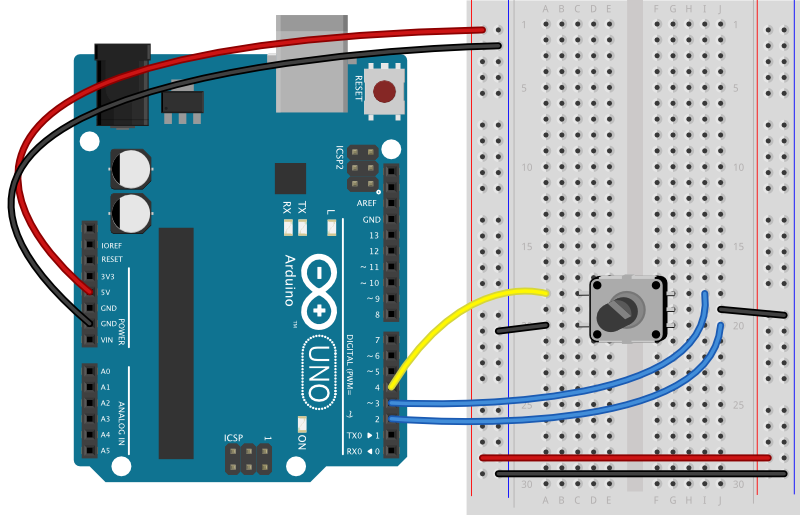
Figure 5. Breadboard view of an Arduino Nano 33 IoT attached to an HC-SR04 ultrasonic sensor. The sensor’s Trigger pin is attached to the Arduino’s digital pin 9, and the sensor’s Echo pin is attached to the Arduino’s digital pin 10. The sensor’s ground is connected to the Arduino’s ground, and the Vcc is attached to either the Arduino’s Vin pin (if the Arduino is powered by USB or other 5V source), or the VUSB pin (if the Arduino is powered by a higher voltage source).
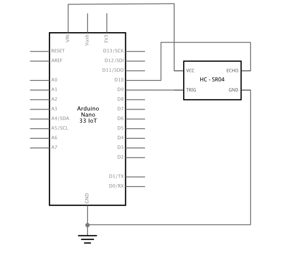
Figure 6. Schematic view of an Arduino Nano 33 IoT attached to an HC-SR04 ultrasonic sensor.
Figures 7 and 8 show the schematic diagram and breadboard layout of the sensor attached to an Arduino Uno. Since the Uno operates on 5V, you can use the +5V output pin from the Uno to power the sensor.
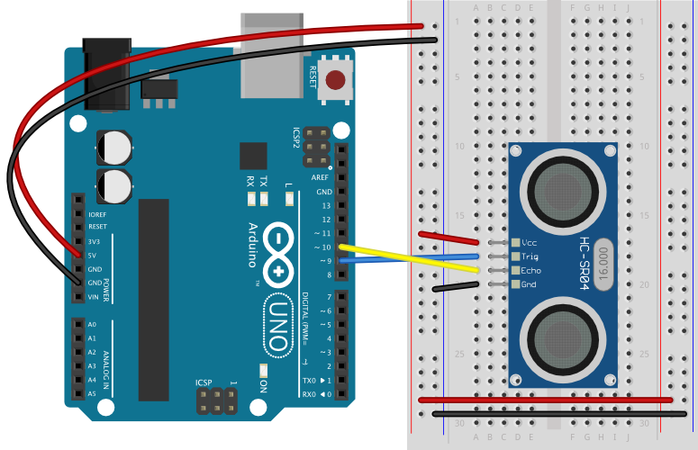
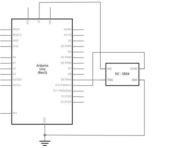
Figure 7. Breadboard view of an Arduino Uno attached to an HC-SR04 ultrasonic sensor. The sensor’s Trigger pin is attached to the Arduino’s digital pin 9, and the sensor’s Echo pin is attached to the Arduino’s digital pin 10. The sensor’s ground is connected to the Arduino’s ground, and the Vcc is attached to the Arduino’s +5V out pin.Figure 8. Schematic view of an Arduino Uno attached to an HC-SR04 ultrasonic sensor. The sensor’s pins are connected to the microcontroller as described in Figure 7.
The Code
The sketch to read the sensor follows the instructions described above. First you take the trigger pin low. Then you take it high to initiate the trigger pulse, then wait ten microseconds. Then you take it low again, ending the trigger pulse. Then you use the pulseIn() command to measure the length of the pulse on the echo pin. After that, you do the math to convert the pulse time to centimeters, and you’re done.
// set up pin numbers for echo pin and trigger pins:
const int trigPin = 9;
const int echoPin = 10;

void setup() {
  // set the modes for the trigger pin and echo pin:
  pinMode(trigPin, OUTPUT);
  pinMode(echoPin, INPUT);
  // initialize serial communication:
  Serial.begin(9600);

}

void loop() {
  // take the trigger pin low to start a pulse:
  digitalWrite(trigPin, LOW);
  // delay 2 microseconds:
  delayMicroseconds(2);
  // take the trigger pin high:
  digitalWrite(trigPin, HIGH);
  // delay 10 microseconds:
  delayMicroseconds(10);
  // take the trigger pin low again to complete the pulse:
  digitalWrite(trigPin, LOW);

  // listen for a pulse on the echo pin:
  long duration = pulseIn(echoPin, HIGH);
  // calculate the distance in cm.
  //Sound travels approx.0.0343 microseconds per cm.,
  // and it's going to the target and back (hence the /2):
  int distance = (duration * 0.0343) / 2;
  Serial.print("Distance: ");
  Serial.println(distance);
  // a short delay between readings:
  delay(10);
}
Clear the Sensing Zone
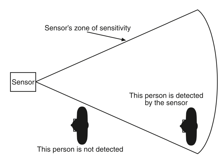
All distance sensors send out their signal and listen for a response in a particular sensing field of view. Figure 9 shows a distance sensor’s typical field of view. The field moves out from the sensor in a cone. It is smaller nearest the sensor, and gets wider as distance from the sensor gets larger. The nearest object in the field of view is the one detected. A person standing outside the field of view cannot be detected by the sensor.
Figure 9. A distance sensor shown from above, with the field of view drawn in. A near person outside the field of view is not detected, while a farther person inside the field of view is detected.
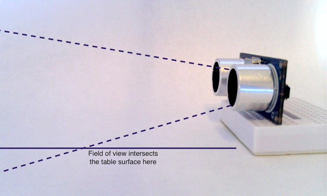
Similarly, an object in the field of view can be detected whether you intend it to or not. Figure 10 shows an ultrasonic sensor sitting on a table. The field of view of the sensor extends out from the sensor, and intersects the table a few centimeters from the sensor. This stops the sensor from picking up more distant targets.
Figure 10. A photo of an ultrasonic sensor sitting on a table. The field of view of the sensor is blocked by the table a few centimeters from the sensor.
Distance sensors can be used for any number of applications including range finding, user detection, and obstacle avoidance. Distance sensors are increasingly commonplace in automobiles to facilitate parking and provide enhanced situational awareness. They are used in smartphones to prevent unintended touchscreen activation when holding the device to your ear, and they are integral to touch free paper towel dispensers. Any camera with autofocus relies on a distance sensor. Whether stationary or in motion, distance sensors take readings using one of three methods: signal strength (how diminished is the emitted signal when reflected off a target); triangulation (distance as a function of the angle at which the emitted signal is reflected off the target); or time of flight (the time it takes for a signal to be emitted, reflected off the target, and received). In this lesson, you’ll learn a few principles of working with these sensors, and see some examples.
What You’ll Need to Know
To get the most out of this page, it helps to be familiar with the following concepts:
It’s important to understand what distance sensors can do, and what they can’t do. Two common uses for distances sensor are measuring distance, or how far away from the sensor a person or object is, and detecting presence, or whether there is a person in front of the sensor at all. Many distance sensors use the term proximity to refer to presence as well. A third use that many people often want from these sensors is to detect attention. Distance and presence or proximity are easy to sense. Attention is a more complex problem, not solved by distance sensors alone. To know whether a sensor can do the job at all, you should also know about where it can sense objects or people. The terms Field of View or Angle of View are often used to describe this in technical documents.
Measuring Distance vs Detecting Presence
“Most sensors that read the distance from a target send out some form of energy (light, magnetism, or sound). They measure the amount of energy that reflects off the target and compare it with the energy that went out. Then they convert the difference into an electrical voltage or digital signal that you can read on a microcontroller… This principle is common to many different sensors and across many scales. On a small scale, domestic robots such as Roombas emit an infrared light and wait for the reflected IR light from an obstacle to navigate a room. On a large scale, airplane radar systems operate by sending out a radio signal and measuring the time it takes for the signal to bounce back from a target….
“One common use for distance sensors is to track a person moving in front of an object in order to trigger the object to action when the person gets close enough. This can be very effective, but keep in mind that being present and paying attention are not the same thing, as any parent or teacher can confirm. Imagine that you want to sense when a person is looking at your painting so that you can make the painting respond in some way. You could put a ranging sensor in front of the painting and look for a person to get close enough, but this sensor alone won’t tell you whether she’s got her back to the painting or not. Sensing attention is a more complex problem.”
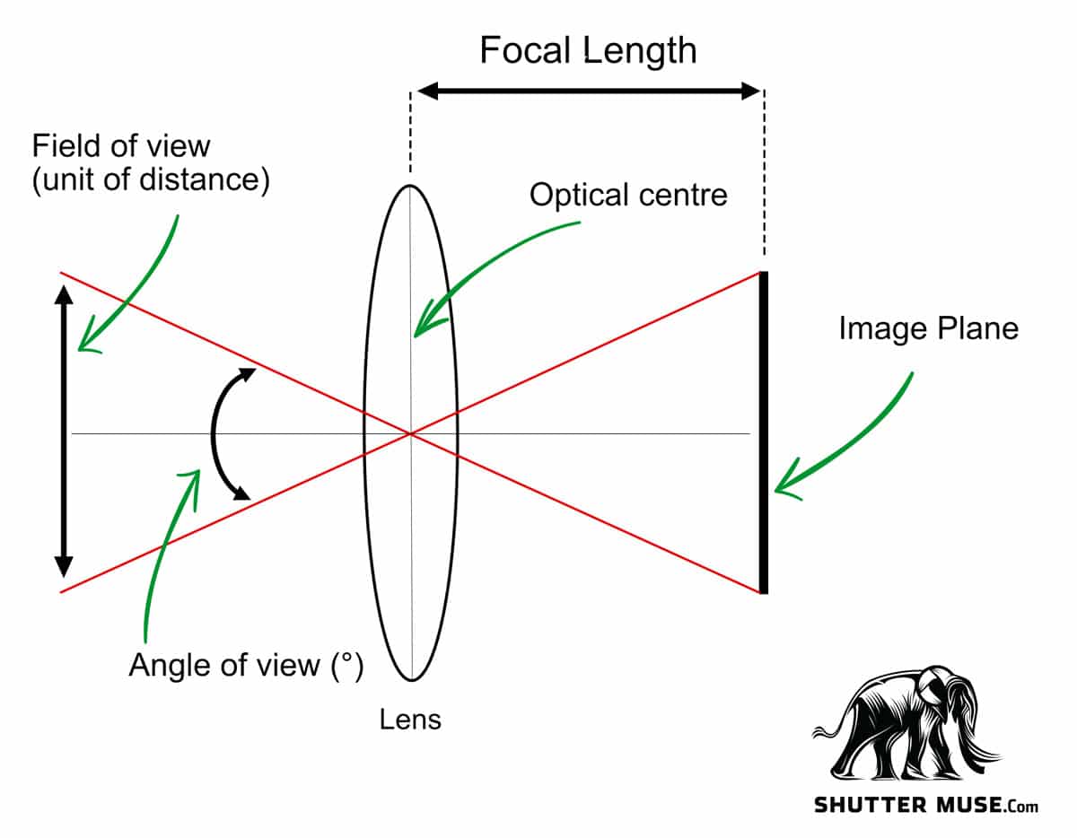
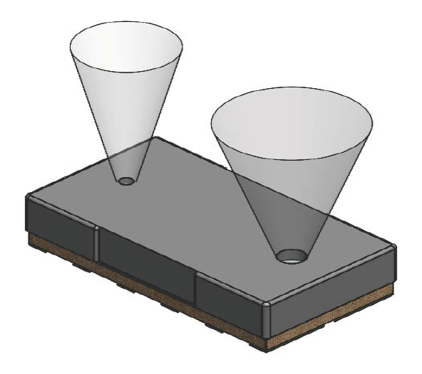
You’ll often see one of two terms referring to a distance sensor’s capabilities: Angle of View or Field of View. While the term “Angle of View” is more accurate, you’ll most often see “Field of View” in documentation for these sensors. Angle of View describes the shape of the cone projected from the sensor within which a signal is either emitted or received and its value is measured in degrees. True Field of View describes the plane perpendicular to the sensor at any given distance that is bounded by the Angle of View. Note that a sensor’s emitter and receiver may have different Angles of View but they are designed to overlap to the greatest extent possible. Figure 1 illustrates the relationship between angle of view and field of view.
Figure 2 shows a typical distance sensor’s two main elements, the emitter and the receiver, showing the the angle of transmission from the transmitter and angle of view from the receiver. They sit beside each other on the device, pointing the same direction.
Whether you’re dealing with an IR proximity sensor, LiDAR distance sensor, or time of flight sensor, there are a few features you’ll need to consider:
Range – Distance sensors come with different minimum and maximum ranges.
Resolution – How granular the units of measurement. Not to be confused with a sensor’s accuracy.
Field of View – More accurately described as Angle of View when measured in degrees, the Field of View describes the area in which a target will trigger a reading at a given distance from the sensor.
Susceptivity to ambient light conditions – With the exception of ultrasonic sensors, the presence of ambient light will affect a distance sensor’s performance. Direct light is more disruptive than indirect, outdoor light more so than indoor, and incandescent light sources more so than artificial.
Some target properties will affect the sensor’s response. For example, large faceted shapes or concave shapes (like the inside of a bowl, or a hat) might not reflect the beam back to the sensor well. Other factors which could affect the response include:
size
orientation (wrt the sensor)
color
transparency
reflectance
texture
Electrical Characteristics – As with any electronic sensor, you should pay attention to current consumption and make sure the rated voltage of your distance sensor is compatible with your microprocessor.
Interface – Distance sensors come with a variety of interfaces. Some provide a changing analog voltage based on range. Others will provide a UART asynchronous or an I2C synchronous serial interface. Ultrasonic distance sensors will provide a changing pulse width that corresponds with the changing properties of the sensor. Nowadays, most light-based distance sensors are I2C.
Extra Features – in addition to the basic physical properties, some distance sensors will have additional features, like the ability to measure ambient light, rudimentary gesture detection, or sophisticated control features like the ability to set angle of view or specific regions of interest (ROI).
Most vendors of sensor modules do not actually make the sensors themselves, they just put them on a breakout board along with the reference circuit, for convenience. While you might buy your distance sensor from Sparkfun, Adafruit, Seeed Studio, or Pololu, for example, the chances are the actual sensor is manufactured by another company like AMS, Sharp, ST Microelectronics, or Vishay. When you shop for a sensor module, check out the manufacturer’s datasheet in addition to the vendor’s tech specs. It’s also worth doing a comparison search with the sensor part number on Octopart.com to see who else might make a breakout board.
Ultrasonic Distance Sensors
Ultrasonic distance sensors use a transducer to emit a pulse of ultrasound at 40 MHz measuring the time it takes for the pulse to bounce off the target and return to the sensor and calculating distance based on the speed of sound. Although it’s unusual to see them described as such, technically they are a sonic time-of-flight sensor. Ultrasonic distance sensors are immune to ambient lighting conditions and target transparency however because sound transmission is influenced by the physical properties of air, accuracy is affected by ambient sound, temperature, and humidity. A ‘soft’ sound absorbing target with a surface covered by cloth will impact accuracy, as will a target with an irregular surface.
HC-SR04 distance sensors are a staple of many starter kits built around the Arduino Uno, which means they are not plug-and-play compatible with 3.3V Arduino boards like the Nano 33 IoT. It’s simple enough to incorporate a voltage divider into your circuit, however, and if you’re feeling adventurous, the HC-SR04 can be permanently modified for use with either 3.3V or 5V logic.
The simplest approach to measuring distance using infrared light is to measure the amount of emitted IR light that bounces off a target and reflects back to the sensor. The ranges are relatively small — between 0 and 20cm — and the language used is ‘proximity’ rather than ‘distance’.
Some optical time-of-flight distance sensors are based on IR LED emitters. They can be pricey. The Benewake TFmini sold by Adafruit, SparkFun and Seeed is capable of ranging distances up to 12 meters and while it requires 5V to operate, it uses 3.3V logic to communicate. Unlike other distance sensors that use I2C, the TFmini uses the UART protocol for asynchronous serial communication.
The Garmin LIDAR-Lite V4 — available at Adafruit and SparkFun (also available with Qwiic connector) — has a 10 meter range and is more expensive than the Benewake sensor but comes with some additional features including I2C serial protocol and wireless control using Garmin’s open ANT Protocol, a low power wireless protocol alternative to BLE.
Note that both Benewake and Garmin take creative license and, while not technically accurate, nonetheless market the two products above as ‘LiDAR’ distance sensors.
Infrared LED Triangulation Sensors
Another method for calculating distance using infrared light is triangulation. A pulse of IR light is emitted and range is determined based on the angle of reflection. Most of the maker / hobbyist sensors of this category are manufactured by Sharp. They come in both analog and digital output variations but because most of them require 5V, they can be used with the Uno but not the Nano 33 IoT. The Sharp GP2Y0A60SZLF is an exception, operating at 3V. Pololu makes a breadboard-friendly module with this sensor.
Maximum distances for analog output sensors range from 5cm to 80cm depending on the model. For sensors with digital output, maximum distances range from 1.5cm to 550cm.
LiDAR Distance Sensors
LiDAR distance ranging sensors like the Garmin LIDAR-Lite v3 available from Adafruit and SparkFun use time-of-flight to calculate distance as a function of the time it takes a pulse of emitted laser light to reflect off a target and return to the sensor. The Garmin LIDAR-Lite v3 is capable of very rapid readings measuring distances up to 40 meters although at a resolution of centimeters rather than millimeters. Data can be sent to the microprocessor as either a digital signal using I2C or an analog signal using pulse width modulation. Distance sensors of this kind are often used in robotics and autonomous vehicles; they are quite expensive and less likely to be of practical use to PComp projects.
LiDAR is an acronym for light detection and ranging pr laser imaging, detection, and ranging. Note that some distance sensors marketed as LiDAR are actually lensed IR LED time-of-flight sensors and do not actually user lasers.
Another example of optical time-of-flight, these distance sensors combine a vertical cavity surface emitting laser (VCSEL) with a single-photon avalanche diode (SPAD) array to measure the time it takes a photon of light to travel from the sensor, to the target, and back. Distance is then calculated using the speed of light, which is a constant. VCSEL distance sensors provide true laser-based ranging with high resolution (millimeters rather than centimeters) in a very small form factor. ST’s VL53L0X and ST’s VL53L1X are VCSEL sensors. A lab exercise on the VL53L0x sensor can be found on this site.
RADAR
RADAR is an acronym for Radio Detection and Ranging. Radar is a technology that dates back to the 1940’s. Despite being a mature technology, though, it is still not as inexpensive or as ubiquitous as other forms of distance ranging. Seeed Studio makes a Doppler Radar module, however, for those interested in radar: Seeed Grove Doppler Radar
What To Look For in a Distance Sensor Library
Different vendors will often write their own libraries for the distance sensors they sell. When you’re looking at a given vendor’s product, take a look at the properties of the sensor in the vendor’s datasheet, and the list of public functions in the library’s API. Does the library give you the functions of the sensor that you need? If the sensor supports multiple sensing ranges, does the library give you access to setting and getting the range? Is it well-documented, and well-commented? Are there simple, clear, well-commented examples?
For example, both SparkFun and Pololu make breakout boards for the VL53L1X Time-of-Flight sensor. The VL53L1X is typical of a next gen distance sensor; it’s got an I2C interface, operates at 2.8V, and offers a large range from 4cm to 400cm. The SparkFun hookup guide is more accessible than the Using the VL53L1X section on Pololu’s product page but neither provides a summary of all the functions in their libraries. To see that, you need to look at the header files for each library.
Pololu offers two different libraries for the VL53L1X. The Pololu VL53L1X library is streamlined to use less resources but doesn’t surface some of the more technical features of the sensor. On the other hand, the Pololu ST VL53L1X API library is a largely literal implementation of ST’s VL53L1X Full API, providing more advanced functionality at the expense of a larger memory footprint and a more opaque code base divided into multiple header files geared less toward the student or hobbyist than someone with an electrical engineering background.
By comparison, SparkFun’s header file is less verbose and significantly shorter than either of the Pololu offerings with clean, succinct, in-line comments that make it accessible and easy to navigate. The public functions start around line 35. Both are functional libraries, though, and you should choose based on the features you want and how easy you find each to use.
You can find further notes on how to pick a library in this lab exercise for the APDS-9960 Color, Light, and Gesture sensor.
Conclusion
There are dozens of distance sensors on the market, and as they become more ubiquitous in electronic devices, they continue to get smaller, cheaper, more sophisticated and more power-efficient. The principles laid out here should give you a basis for assessing new sensors as needed.
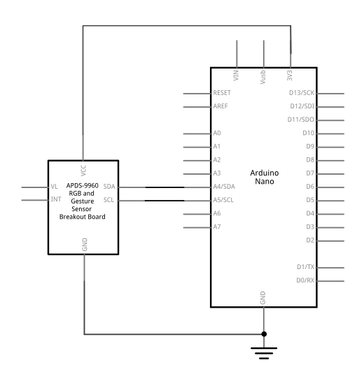
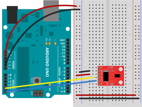
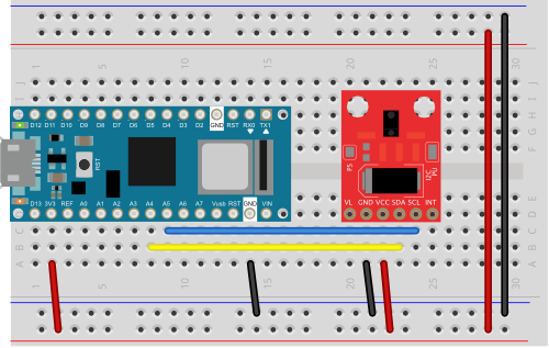
In this lab, you’ll see synchronous serial communication in action using the Inter-integrated Circuit (I2C) protocol. You’ll communicate with a color, gesture, and proximity sensor from a microcontroller.
Introduction
In this lab, you’ll see synchronous serial communication in action using the Inter-integrated Circuit (I2C) protocol. You’ll communicate with a color, gesture, and proximity sensor from a microcontroller.
There are many different sensors on the market that use the I2C protocol to communicate with microcontrollers. It is the most common way to connect to sensors these days. The one used in this lab is typical, so the I2C principles covered here will help you when working with other I2C sensors as well.
Figure 1-3 are the parts that you need for this lab.
Figure 1. 22AWG solid core hookup wires.
Figure 2. Arduino Nano 33 IoT or other Arduino board
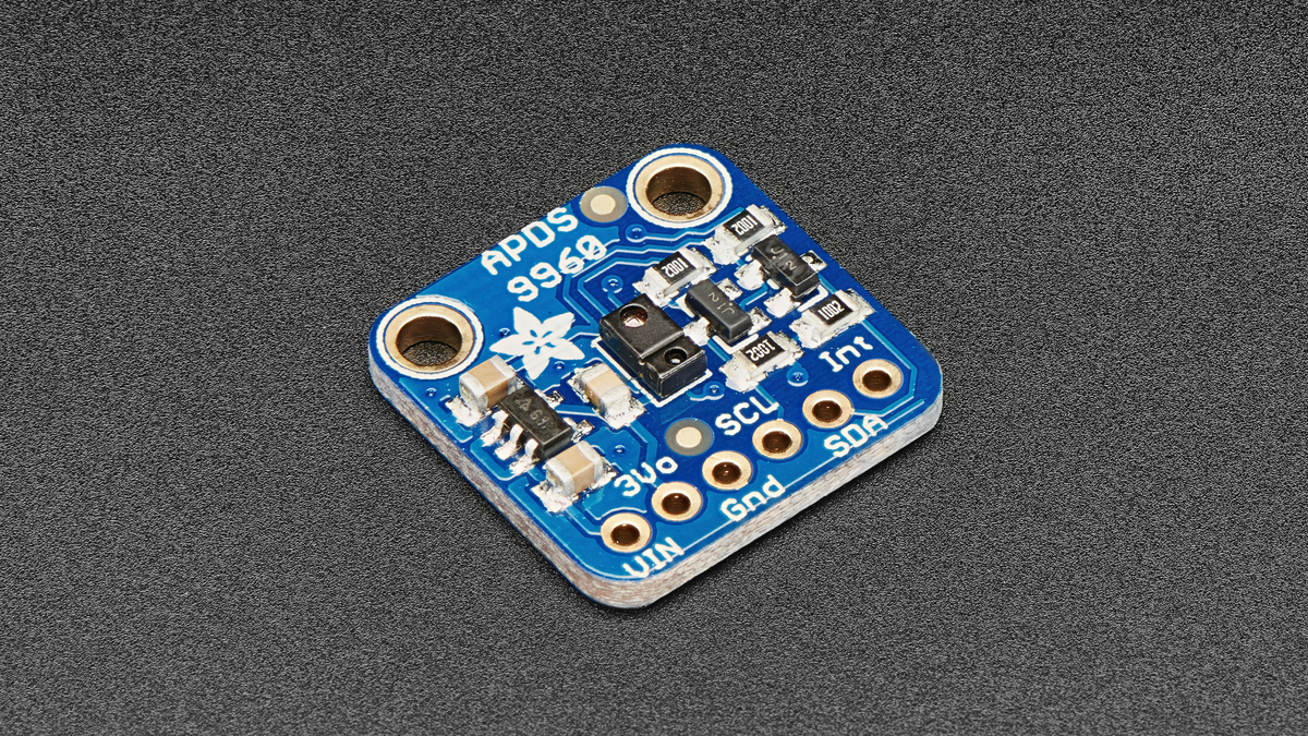
Figure 3. An APDS-9960 color and gesture sensor breakout board.
Sensor Characteristics
The sensor used in this lab, a Broadcom APDS-9960 sensor, is an integrated circuit (IC) that can read the color of an object placed in front of it; proximity, within about 10cm; and gestures on the axes parallel to the sensor (up, down, left, and right). It senses color using four photodiodes, three of which have color filters (red, green, and blue) and one of which has no filter (clear). The color sensors are filtered to block IR and UV light. It senses gesture using four directional photodiodes, picking up reflected IR energy from a built-in IR LED. The combination of sensors is used to determine the direction of an object moving above the board, and its proximity.
The company that makes this sensor, Broadcom, doesn’t make their own breakout boards, but a few other companies do. There’s a breakout board available from Sparkfun and one from Adafruit and one from DFRobot (all available through Digikey) and there’s an APDS9960 sensor built into the Arduino Nano 33 BLE Sense board as well.
I2C Connections
Connect the sensor’s voltage and ground connections to your voltage and ground buses, and the connections for I2C clock (SCL) and I2C serial data (SDA) as shown in Figure 4-6. The schematic, Figure 4, is the same for both the Uno and the Nano. For the Arduino Uno or the Arduino Nano boards, the I2C pins are pins A4 (SDA) and A5(SCL). This is the same connection for almost any I2C sensor.
Some I2C sensors also have a few other pins:
an interrupt pin, which they use to signal the microprocessor when a reading is ready. The APDS-9960 has an interrupt pin, but you don’t have to use it if you don’t want to. Your code will need to change if you use the interrupt. You can read more about that later in this lab.
a shutdown or reset pin, which can be used for powering down or resetting the sensor. This sensor doesn’t have that pin.
What are Qwiic/Stemma/Grove/Gravity?
In addition to the standard I2C connections, Sparkfun and Adafruit use a connector called Qwiic which connects the I2C, power, and interrupt connectors all in one cable, eliminating the need for soldering. It’s a Sparkfun brand name. However, you’ll need a Qwiic adapter shield to use it. Adafruit have a similar brand called Stemma, Seedstudio uses Grove, and DFRobot uses Gravity. They all support I2C, and they all have custom solderless connectors, though they are not all compatible with each other. The most compatible way is to stick with the I2C header pins.
Figure 4. Schematic view of an Arduino attached to an APDS-9960 sensor.
Figure 5. Breadboard view of an Arduino attached to an APDS-9960 sensor. This shows a Sparkfun breakout board, but the other companies’ boards use the same pins: voltage, ground, SDA, and SCL.
Figure 6. An APDS-9960 color sensor breakout board connected to an Arduino Nano 33 IoT. This shows a Sparkfun breakout board, but the other companies’ boards use the same pins: voltage, ground, SDA, and SCL.
The circuit is now complete, and you’re ready to write a program to control it. One of the advantages of the I2C synchronous serial protocol (as opposed to the SPI protocol) is that you only ever need two wires for communication to one or multiple devices.
How I2C Sensors Work
I2C devices exchange bits of data whenever the shared clock signal changes. Controller and peripheral devices both send bits of data when the clock changes from low to high (called the rising edge of the clock). Unlike with SPI, they cannot send data at the same time.
The APDS-9960 has a series of memory registers that control its function. You can write to or read from these registers using I2C communication from your microcontroller. Some of these registers are writable by the controller so that you can configure the sensor. For example, you can set set the sensitivity of the sensor, and so forth. Some registers are configuration registers, and by writing to them, you configure the chip. For example, you can set lower and upper limits of temperature sensitivity. Other memory registers are read-only. For example, when the sensor has read the proximity of an object, it will store the result in a register that you can read from the controller. The details of the chip’s registers can be found in thesensor’s datasheet.
How I2C Bits are Exchanged
Most of the time, you never have to think about how the bits of an I2C message are exchanged, and the next section, I2C Libraries, will be more important to you. For the low-level details, read on:
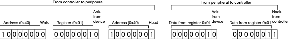
I2C devices exchange data in 7-bit chunks, using an eighth bit to signal if you’re reading or writing by the controller or for acknowledgement of data received. To get the temperature from the APDS-9960, your controller device sends the sensor’s address (a 7-bit number, for this sensor it’s 0×39) followed by a single bit indicating whether you want to read data or write data (1 for read, 0 for write). This means that the 8-bit byte sent is actually 0x72 or 0x73, depending on the state of the read/write bit. Then you send the memory register that you want to read from or write to. For example, as shown in Figure 7, the proximity reading is stored in memory register 0x9C of the APDS9960. To get the proximity, you send 0x72 (0x39 shifted up one bit, with 0 in the R/W bit); then 0x9C for the register you want to read. The response in this case is 0x77. The bottom bit is a 1, meaning no ACK was sent from the sensor. That converts to a proximity reading of 118.
Figure 7. I2C data
I2C and the Wire Library
To use I2C communication on an Arduino microcontroller, you use the Wire library, which is built into the Arduino IDE. You can find Arduino-compatible libraries for many devices that use the Wire library, but never expose it directly in their APIs. The libraries for this sensor are typical of this style of library. For example, the Arduino_APDS9960 library’s readColor() command sends a write command to start a reading of the sensor’s color photodiodes. The colorAvailable() sends a read command to read the register that indicates whether or not the color reading is done.
All sensors take a certain amount of time to read the physical phenomena which they sense. With light-based sensors like the APDS-9960, the time they take to get a reading is usually called integration time, and it’s noted in the data sheet how long it is (page 4). The color sensor of the APDS-9960 has an integration time of between 2.78ms and 708ms, depending on your settings. In operation, you query the sensor as to whether it’s got a reading available, and then read it when that’s true.
How To Pick a Library
Most every company that makes a breakout board for a given I2C sensor will also write a library for it. For example, there’s the Arduino_APDS9960, the SparkFun_APDS9960, and the Adafruit_APDS9960 library. All three of these will work with any of the three breakout boards. The Arduino Nano 33 BLE sense will only work with the Arduino_APDS9960 library. Otherwise, what’s the difference?
Different companies and programmers have different styles for writing a library’s application programming interface, or API. Arduino has a style guide for writing APIs, but it’s not always followed by others. The Arduino_APDS9960 library follows this guide, and has the simplest API of the three. The Sparkfun_APDS9960 offers a few more configuration functions, as does the Adafruit_APDS9960, and their examples are a bit more complicated as a result. You should look at the examples with any library to see if they make sense to you. A good guideline is to use the library with the instructions and examples that you find to be the clearest. It’s also good to check the company’s guide to the sensor if they have one. Here are the guides for this sensor: Sparkfun Hookup guide; Adafruit guide; Arduino library reference.
You can also get information from the library’s header file. The header file is generally the file with the name libraryname.h. Sometimes it’s in a directory called src. For example, here’s the header file for the Arduino_APDS9960 library. Here’s the one for the Sparkfun library and the one for the Adafruit library. Within the header file, there’s a class names for the library and a section called public where all the possible function definitions are.
Even if the examples don’t include all the functions, the public section of the header file will. From there, you can build your own examples if the library’s examples don’t show how to use a function you want to use.
All three libraries operate in more or less the same way, because they have to access the same functions of the sensor. They start the function (color, proximity, or gesture) using an enable function in the setup. In the main loop, they query the sensor if it’s got a reading, and then read it if it does. For example, to use the color function, the Arduino and Adafruit libraries have functions that check if the sensor’s got a good reading: colorDataReady() in the Adafruit library and colorAvailable() in the Arduino library. The Sparkfun has no function like this, so you have to add a delay between color readings.
The Sparkfun and Adafruit libraries provide functions to explicitly enable or disable the sensor’s three major functions. The Arduino library does this work implicitly by enabling each function when you call the available() functions, and disabling the function after each read. The former give you more control, but require you to make sure you’ve done the enabling and disabling. The latter is more automatic, but gives you less discrete control.
Install the External Libraries
You can use the library manager to find these libraries. Make sure you’re using Arduino version 1.8.9 or later. From the Sketch menu, choose Include Library, then Manage Libraries, and search for APDS9960. All three of the libraries mentioned here will show up. The examples below use the Arduino_APDS9960 library, as it’s the simplest of the three.
Program the Microcontroller
At the beginning of your code, include the appropriate libraries. In the setup(), initialize the sensor with a function called begin() (Sparkfun sometimes uses init() instead of begin()). If the sensor responds, then begin() will return true, and if not, it will return false. This is how to check that the sensor is properly wired to your microcontroller:
#include "Arduino_APDS9960.h"

void setup() {
  Serial.begin(9600);
  // wait for Serial Monitor to open:
  while (!Serial);
  // if the sensor doesn't initialize, let the user know:
  if (!APDS.begin()) {
    Serial.println("APDS9960 sensor not working. Check your wiring.");
    // stop the sketch:
    while (true);
  }

  Serial.println("Sensor is working");
}
In the main loop() function, you’ll read the sensors. Here’s how to read the color sensor using the Arduino_APDS9960 library. You’re going to query the sensor to see if it’s got a reading available with the available() function, then you’ll use the read() function to get the result:
void loop() {
  // red, green, blue, clear channels:
  int r, g, b, c;

  // if the sensor has a reading:
  if (APDS.colorAvailable()) {

    // read the color
    APDS.readColor(r, g, b, c);

    // print the values
    Serial.print(r);
    Serial.print(",");
    Serial.print(g);
    Serial.print(",");
    Serial.print(b);
    Serial.print(",");
    Serial.println(c);
  }
}
You can run this sketch now, and it will print out values for red, green, blue, and clear channels, like so (Here’s a link to the full sketch):
Sensor is working
17,12,16,40
17,12,16,41
17,12,16,41
17,12,16,41
17,12,16,41
17,12,16,40
16,12,16,40
16,11,15,39
As you can see, you’re never actually calling commands from the Wire library directly, but the commands in the sensor’s library are relying on the Wire library. This is a common way to use the Wire library to handle I2C communication. If you’re looking for more examples with this sensor, the libraries all come with examples when you install them. There are some other examples for this sensor in the github repository for this class, using all three libraries. There are two important things to note:
None of the three libraries give light readings in lux, or proximity readings in millimeters.
All of the libraries are controlling the same sensor, and therefore can yield the same results. You may need to configure the sensor differently for each library though. Check the header files for each library (Arduino, Adafruit, Sparkfun) to learn their configuration functions, and check the data sheet to learn more about the sensor’s characteristics.
Using the Sensor’s Interrupt
Most I2C sensors include an interrupt pin. This pin can be used to signal the microcontroller when something important happens, like when the sensor has a good reading, or when the sensor reading crosses a particular threshold. Using the interrupt means that as soon as the sensor is ready to give you a reading, it interrupts the microcontoller.
The interrupt pin for an I2C sensor is usually configurable through the sensor’s API. For example, with the Sparkfun and Adafruit libraries for this sensor you can set the interrupt to signal when any of the three functions changes significantly, and with the Sparkfun library you can set the low and high thresholds for the proximity function.
For basic use of most sensors, you don’t need the interrupt, for for advanced use, it can be helpful. For more on using interrupts, see the Arduino reference page on interrupts.
Conclusion
I2C is a common protocol among many ICs, and it’s handy because you can combine many devices on the same bus. You need to make sure the device addresses are unique. Some devices will have fixed addresses, so that you can’t use multiples of the same sensor together. Others will have a way to change the address. For the APDS9960, the address is fixed.
In this exercise you’ll read the built-in Inertial Motion Unit on the Arduino Nano 33 IoT, then feed its output into a Madgwick filter to determine heading, pitch, and roll of the board. Then you’ll send the output of that serially to p5.js and use it to move a virtual version of the Nano onscreen.
Introduction
In this exercise you’ll read the built-in Inertial Motion Unit on the Arduino Nano 33 IoT, then feed its output into a Madgwick filter to determine heading, pitch, and roll of the board. Then you’ll send the output of that serially to p5.js and use it to move a virtual version of the Nano onscreen.
What You’ll Need to Know
To get the most out of this lab, you should be familiar with the following concepts and you should install the Arduino IDE on your computer. You can check how to do so in the links below:
The only part you’ll need for this exercise is an Arduino Nano 33 IoT and its built-in IMU, as shown in Figure 1. You can modify this exercise to work with other IMUs, however. There are details on various IMUs on the accelerometers, gyrometers, and IMUs page.
Figure 1. Microcontroller. Shown here is an Arduino Nano 33 IoT.
Prepare the Breadboard
because the Nano 33 IoT has a built-in IMU, there is no additional circuit needed for this exercise. However, there are two libraries you’ll need to install: the Arduino_LSM6DS3 library, which allows you to read the IMU, and the MadgwickAHRS library, which takes the raw accelerometer and gyrometer inputs and provides heading, pitch, and roll outputs. Both libraries can be found in the Library Manager of the Arduino IDE. Install them before proceeding.
Program the Microcontroller to Read the IMU
The first thing to do in the microcontroller code is to confirm that your accelerometer and gyrometer are working. Start with the code below:
#include "Arduino_LSM6DS3.h"

void setup() {
  Serial.begin(9600);
  // attempt to start the IMU:
  if (!IMU.begin()) {
    Serial.println("Failed to initialize IMU");
    // stop here if you can't access the IMU:
    while (true);
  }
}

void loop() {
  // values for acceleration and rotation:
  float xAcc, yAcc, zAcc;
  float xGyro, yGyro, zGyro;

  // check if the IMU is ready to read:
  if (IMU.accelerationAvailable() && IMU.gyroscopeAvailable()) {
    // read accelerometer and gyrometer:
    IMU.readAcceleration(xAcc, yAcc, zAcc);
    IMU.readGyroscope(xGyro, yGyro, zGyro);

    Serial.print("sensors: ");
    Serial.print(xAcc);
    Serial.print(",");
    Serial.print(yAcc);
    Serial.print(",");
    Serial.print(zAcc);
    Serial.print(",");
    Serial.print(xGyro);
    Serial.print(",");
    Serial.print(yGyro);
    Serial.print(",");
    Serial.println(zGyro);
  }
}
When you run this sketch and open the Serial Monitor, you should see a printout with six values per line. The first three are your accelerometer values, and the next three are your gyrometer values. The following reading is typical:
sensors: 0.04,-0.05,1.02,3.05,-3.72,-1.77
The Nano 33 IoT’s accelerometer’s range is fixed at +/-4G by this library, and its gyrometer’s range is set at +/-2000 degrees per second (dps). The sampling rate for both is set to 104 Hz by the library. Other IMUs may have differing ranges. You need to know at least the sampling rate when you want to use a different IMU with this exercise. If you know that information, though, it’s easy to swap one IMU for another in the Madgwick library.
Add the Madgwick Library to Get Orientation
The MadgwickAHRS library can work with any accelerometer/gyrometer combination. It expects the acceleration in Gs and the rotation in degrees per second as input, and uses the sensors’ sampling rate when you initialize it. Add a few lines to the code before your setup() as follows:
#include "Arduino_LSM6DS3.h"
#include "MadgwickAHRS.h"

// initialize a Madgwick filter:
Madgwick filter;
// sensor's sample rate is fixed at 104 Hz:
const float sensorRate = 104.00;

// values for orientation:
float roll = 0.0;
float pitch = 0.0;
float heading = 0.0;
Next, add the following line at the end of the setup() to initialize the Madgwick filter:
// start the filter to run at the sample rate:
filter.begin(sensorRate);
Now change the main loop so that you’re sending the sensor readings into the Madgwick filter. You’ll do this inside of the if statement that checks if the sensors are ready:
// check if the IMU is ready to read:
if (IMU.accelerationAvailable() &&
IMU.gyroscopeAvailable()) {
  // read accelerometer and gyrometer:
  IMU.readAcceleration(xAcc, yAcc, zAcc);
  IMU.readGyroscope(xGyro, yGyro, zGyro);

  // update the filter, which computes orientation:
  filter.updateIMU(xGyro, yGyro, zGyro, xAcc, yAcc, zAcc);

  // print the heading, pitch and roll
  roll = filter.getRoll();
  pitch = filter.getPitch();
  heading = filter.getYaw();

  // print the filter's results:
  Serial.print(heading);
  Serial.print(",");
  Serial.print(pitch);
  Serial.print(",");
  Serial.println(roll);
}
Now when you run the sketch, you’ll get heading, pitch, and roll instead of the raw sensor readings. Here’s a typical output you might see:
167.59,-2.50,-2.52In this case, the readings are all in degrees. The first is the heading angle, around the Z axis. The second two are the pitch, around the x axis, and roll, around the Y axis.
Add Serial Handshaking
Reading these values in p5.js will work smoother if you add handshaking, also known as call-and-response, to your serial communications protocol. Modify the loop() so that the sketch sends the latest heading, pitch, and roll whenever a new byte comes in the serial port. Here’s the final version of the loop():
void loop() {
  // values for acceleration and rotation:
  float xAcc, yAcc, zAcc;
  float xGyro, yGyro, zGyro;

  // check if the IMU is ready to read:
  if (IMU.accelerationAvailable() & amp; & amp;
      IMU.gyroscopeAvailable()) {
    // read accelerometer and gyrometer:
    IMU.readAcceleration(xAcc, yAcc, zAcc);
    IMU.readGyroscope(xGyro, yGyro, zGyro);

    // update the filter, which computes orientation:
    filter.updateIMU(xGyro, yGyro, zGyro, xAcc, yAcc, zAcc);

    // print the heading, pitch and roll
    roll = filter.getRoll();
    pitch = filter.getPitch();
    heading = filter.getYaw();
  }

  // if you get a byte in the serial port,
  // send the latest heading, pitch, and roll:
  if (Serial.available()) {
    char input = Serial.read();
    Serial.print(heading);
    Serial.print(",");
    Serial.print(pitch);
    Serial.print(",");
    Serial.println(roll);
  }
}
this link. When you have this much working, and you’ve tested it in the Serial Monitor, you can close Arduino and work on the p5.js sketch.
Program p5.js to Read the Incoming Serial Data
Now it’s time to write a p5.js sketch to read this data. The setup will be the same as it was in the Serial Input to p5.js using WebSerial lab. The checklist from that lab lays out all the important parts you need.
Make a P5.js sketch. If you’re using the p5.js web editor, make a new sketch. Click the Sketch Files tab, and then choose the index.html file. Edit the head of the document as you did for the other p5.webserial labs. It should look like this:
Start your sketch with some code to initialize the serial library:
// variable to hold an instance of the p5.webserial library:
const serial = new p5.WebSerial();

// HTML button object:
let portButton;

function setup() {
  	createCanvas(500, 600, WEBGL);     // make the canvas
  // check to see if serial is available:
  if (!navigator.serial) {
    alert("WebSerial is not supported in this browser. Try Chrome or MS Edge.");
  }
  // if serial is available, add connect/disconnect listeners:
  navigator.serial.addEventListener("connect", portConnect);
  navigator.serial.addEventListener("disconnect", portDisconnect);
  // check for any ports that are available:
  serial.getPorts();
  // if there's no port chosen, choose one:
  serial.on("noport", makePortButton);
  // open whatever port is available:
  serial.on("portavailable", openPort);
  // handle serial errors:
  serial.on("requesterror", portError);
  // handle any incoming serial data:
  serial.on("data", serialEvent);
  serial.on("close", makePortButton);
}
function draw() {

}

// if there's no port selected,
// make a port select button appear:
function makePortButton() {
  // create and position a port chooser button:
  portButton = createButton('choose port');
  portButton.position(10, 10);
  // give the port button a mousepressed handler:
  portButton.mousePressed(choosePort);
}

// make the port selector window appear:
function choosePort() {
  serial.requestPort();
}

// open the selected port, and make the port
// button invisible:
function openPort() {
  // wait for the serial.open promise to return,
  // then call the initiateSerial function
  serial.open().then(initiateSerial);

  // once the port opens, let the user know:
  function initiateSerial() {
    console.log("port open");
    serial.write("x");
  }
  // hide the port button once a port is chosen:
  if (portButton) portButton.hide();
}

// read any incoming data:
function serialEvent() {
  // read a string from the serial port
  // until you get carriage return and newline:
  var inString = serial.readStringUntil("\r\n");
  console.log(inString);
}

// pop up an alert if there's a port error:
function portError(err) {
  alert("Serial port error: " + err);
}

// try to connect if a new serial port
// gets added (i.e. plugged in via USB):
function portConnect() {
  console.log("port connected");
  serial.getPorts();
}

// if a port is disconnected:
function portDisconnect() {
  serial.close();
  console.log("port disconnected");
}
Save this as sketch.js, then open p5.serialcontrol. Then open the sketch in a browser. Open the JavaScript console, and you should see the first set of data printed out. This is because the initiateSerial() function sent a single byte to the Nano when the port opened, and the Nano sent one set of readings. That generated a serial data event in p5.js, and called the serialEvent() function, which printed out the results.You need this to happen repeatedly: p5.js sends a byte when it wants new data, then the Nano sends the data, then waits for another byte from p5.js.
Add Serial Handshaking
To make this happen, you need to add a few things to your p5.js sketch. You can assume that if you saw the message in the console, then you’re ready for new data. That’s when you should send a byte back to the microcontroller to request new data. Add one line to the serialEvent() function to make this happen:
// callback function for incoming serial data:
ffunction serialEvent() {
  // read a string from the serial port
  // until you get carriage return and newline:
  var inString = serial.readStringUntil("\r\n");
  if (inString != null) {
    console.log(inString);
    serial.write("x");
  }
}
When you run the sketch with this update, you should see a continuous flow of new data from the microcontroller.
Next, you need to break the string up into parts and convert them into floating point numbers so you can use them as heading, pitch, and roll. Start by adding three new variables at the top of your sketch as global variables, because you’ll need them when you draw the virtual Arduino:
// orientation variables:
let heading = 0.0;
let pitch = 0.0;
let roll = 0.0;
Next, in the serialEvent() function, use the JavaScript trim() function to get rid of any extraneous characters at the end of the message string, like carriage returns or newlines. Then use the split() function to split the string into a list of elements separated by commas. Then convert them to floating point numbers. Once you know you have three valid numbers for heading, pitch, and roll, send another byte to the microcontroller to get a new reading. Here’s what the new version of serialEvent() looks like:
function serialEvent() {
  // read from port until new line:
  let inString = serial.readStringUntil("\r\n");
  if (inString != null) {
    let list = split(trim(inString), ",");
    if (list.length > 2) {
      // conver list items to floats:
      heading = float(list[0]);
      pitch = float(list[2]);
      roll = float(list[1]);
      console.log(heading + "," + pitch + "," + roll);
      // send a byte to the microcontroller to get new data:
      serial.write("x");
    }
  }
}
When you reload the sketch after making these changes, you should be getting floating point numbers for heading, pitch and roll. Once you have these values coming in consistently, it’s a good idea to comment out the console.log() statement, as shown above, as it slows down the sketch considerably.
Now that you have serial communication working properly, it’s time to write the code to draw the virtual microcontroller.
Draw the Virtual Arduino
Add the function below to draw a virtual Arduino. It draws in three dimensions, using the WEBGL framework you chose in createCanvas() above in the setup() function.
// draws the Arduino Nano:
function drawArduino() {
   // the base board:
   stroke(0, 90, 90); // set outline color to darker teal
   fill(0, 130, 130); // set fill color to lighter teal
   box(300, 10, 120); // draw Arduino board base shape

   // the CPU:
   stroke(0);         // set outline color to black
   fill(80);          // set fill color to dark grey
   translate(30, -6, 0); // move to correct position
   box(60, 0, 60);    // draw box

   // the radio module:
   stroke(80);       // set outline color to grey
   fill(180);        // set fill color to light grey
   translate(80, 0, 0); // move to correct position
   box(60, 15, 60);  // draw box

   // the USB connector:
   translate(-245, 0, 0); // move to correct position
   box(35, 15, 40);	  // draw box
}
You haven’t added a draw() function yet, so add it now, as follows:
function draw() {
   background(255); // set background to white
   push();          // begin object to draw
   // draw arduino board:
   drawArduino();
   pop();           // end of object
}
When you reload the sketch, you’ll see a drawing like that in Figure 4. It won’t change.
Figure 4. A virtual Arduino Nano 33 IoT, drawn in in p5.js. The Nano is seen from the side, with the USB connector on the right, and the radio on the right.
To make it change its orientation, you need to use the heading, pitch, and roll values to rotate the object. You get the sine and cosine of each angle, and use them to generate a matrix for translation. The math below was worked out by Helena Bisby based on the Madgwick algorithm. p5.js’ applyMatrix() function does the matrix math for you to rotate in all three dimensions. Modify the draw() function as shown below:
function draw() {
   // update the drawing:
   background(255); // set background to white
   push();          // begin object to draw

   // variables for matrix translation:
   let c1 = cos(radians(roll));
   let s1 = sin(radians(roll));
   let c2 = cos(radians(pitch));
   let s2 = sin(radians(pitch));
   let c3 = cos(radians(heading));
   let s3 = sin(radians(heading));
   applyMatrix(c2 * c3, s1 * s3 + c1 * c3 * s2,
      c3 * s1 * s2 - c1 * s3, 0, -s2, c1 * c2,
      c2 * s1, 0, c2 * s3, c1 * s2 * s3 - c3 * s1,
      c1 * c3 + s1 * s2 * s3, 0, 0, 0, 0, 1);

   // draw arduino board:
   drawArduino();
   pop(); // end of object
}
When you reload the sketch after making these changes, the virtual Arduino should change its position as you move the physical Arduino. That’s the whole application! Figure 5 shows the virtual Arduino in motion.
You can see the sketch running on GitHub at this link. You can see the source files for copying into the p5.js editor at this link.
Figure 5. This virtual Arduino Nano, written in p5.js, moves in three dimensions as you move a real Nano connected to the sketch serially.
Conclusion
If you followed along all of the steps to this application, you probably hit a number of places where communication broke down. There are a lot of pieces to this application, and they all need to work together.
Get the Sensors Working
When you’re dealing with IMU sensors, no data will be perfect, because the sensor’s measurement is always relative. You’ll notice, for example, that the position of the virtual Arduino drifts a bit the longer you run the sketch. Heading, in particular, tends to drift. In real-world applications, this is often adjusted by using a magnetometer as a compass in addition to the accelerometer and gyrometer. It’s also wise to provide ways for a human to calibrate the system, perhaps by pressing a button when the sensor is level in order to calculate offset values for the sensors. For many interactive applications, though, even an imperfect measurement of orientation will do the job well.
Test the Hardware
If you’re using serial communication that’s ASCII-encoded like this, you can always use the Serial Monitor or another serial terminal application to test the Arduino sketch before you ever begin working on the multimedia programming. Ideally, you don’t need to change the Arduino sketch at all once your communication is working as planned.
Get the Communication Working
Whenever you’re building an application that incorporates asynchronous serial communication, it’s best to get the communication working correctly before you build the animation or other parts of the interaction. Once the communication protocol is known, you can even divide the work, with one team developing the hardware and another developing the media programming.
This exercise shows the value of using handshaking (aka call-and-response) in serial communication. Because the drawing of the microcontroller takes time, the p5.js sketch reads data less frequently than the microcontroller can send it. If you simply allow the microcontroller to send data continuously, the serial buffer on the p5.js side will fill up, and the movement of the virtual Arduino will become sluggish. This is why you only send back to the microcontroller when you know you have a set of valid data, in the serialEvent() function.
Test the Incoming Data
You don’t need to do anything with your incoming serial data to know it’s valid, if you’ve thought through the protocol well. In this case, if you see you’re getting three separate values and they’re all in a range of 0 to 360 (indicating degrees of the heading, pitch, and roll angles), you know it’ll work.
Program the Interface, Animation, etc.
Once you know the communication is good, and you’re getting accurate values, you can program the parts of your final application that use that data. In this case, you didn’t even start on the movement of the virtual Arduino until you knew you had communication working. Drawing of the virtual model was separated from moving it, using the push(), pop(), and translation functions, like applyMatrix(), in p5.js. That separation makes the programming easier to do, and easier to debug.
Inertial Motion Units (IMUs) are sensors that measure movement in multiple axes. Accelerometers measure a changing acceleration on the sensor. They can be used to measure the tilt of the sensor with respect of the Earth, or the force of a hit. They are common in mobile devices and automobiles. Gyrometers measure changing angular motion. They can be used to measure rotation. Magnetometers measure the magnetic force on a sensor. These are usually used to measure the Earth’s gravitational field in order to determine compass heading. IMUs have become increasingly common in microcontroller projects, to the point where they are built into some microcontroller boards like the Arduino 33 IoT and BLE Sense, and the Arduino 101. In this lesson, you’ll learn a few principles of working with these sensors, and see some examples.
What You’ll Need to Know
To get the most out of this lab, you should be familiar with the following concepts and you should install the Arduino IDE on your computer. You can check how to do so in the links below:
Figures 1-4 below show the parts you’ll need for this exercise. Click on any image for a larger view.
Figure 1. Microcontroller. Shown here is an Arduino Nano 33 IoT. An Uno will do for some of the examples here, though.
Figure 2. Jumper wires. You can also use pre-cut solid-core jumper wires.
Figure 3. A solderless breadboard
Figure 4. An accelerometer. Shown here is an ST Microelectronics LIS3DH accelerometer. Others will be mentioned below.
Orientation, Position, and Degrees of Freedom
“Orientation, or compass heading, is how you determine your direction if you’re level with the earth. If you’ve ever used an analog compass, you know how important it is to keep the compass level in order to get an accurate reading. If you’re not level, you need to know your tilt relative to the earth as well. In navigational terms, your tilt is called your attitude, and there are two major aspects to it: roll and pitch. Roll refers to how you’re tilted side-to-side. Pitch refers to how you’re tilted front-to-back.
“Pitch and roll are only two of six navigational terms used to refer to movement. Pitch, roll, and yaw refer to angular motion around the X, Y, and Z axes. These are called rotations. Surge, sway, and heave refer to linear motion along those same axes. These are called translations. These are often referred to as six degrees of freedom. Degrees of freedom refer to how many different parameters the sensor is tracking in order to determine your orientation.
“You’ll hear a number of different terms for these sensors. The combination of an accelerometer and gyrometer is sometimes referred to as an inertial measurement unit, or IMU… When an IMU is combined with a magnetometer, the combination is referred to as an attitude and heading reference system, or AHRS. Sometimes they’re also called magnetic, angular rate, and gravity, or MARG, sensors. You’ll also hear them referred to as 6-degree of freedom, or 6-DOF, sensors. There are also 9-DOF sensors that incorporate all three types of sensors. Each axis of measurement is another degree of freedom. [There are] even has 10-DOF sensor[s] that add barometric pressure sensor[s] for determining altitude.”
Whether you’re dealing with an accelerometer, gyrometer, or magentometer, there are a few features you’ll need to consider:
Range – IMU sensors come in different ranges of sensitivity.
Acceleration is generally measured in meters per second squared (m/s^2) or g’s, which are multiples of the acceleration due to gravity. 1g = 9.8 m/s^2. Accelerometers come in ranges from 2g to 250g and beyond. the force of gravity is 1g, but a human punch can be upwards of 100g
Angular motion is measured in degrees per second (dps). Gyro ranges of 125dps to 2000 dps are not uncommon.
Magnetic force is measured in Teslas. In most direction applications, the important measurement, however is the relative magnetic field strength on each axis.
Number of axes – Almost all IMU sensors can sense their respective properties on multiple axes. Whatever activity you’re measuring, you’ll most likely want to know the acceleration, rotational speed, or magnetic force in horizontal and vertical directions. Most sensors give results for the X, Y, and Z axes. Z is typically perpendicular to the Earth, and the other two are parallel to it, but perpendicular to each other.
Electrical Characteristics – as with any electronic sensor, you should pay attention to current consumption and make sure the rated voltage of your IMU is compatible with your microcontroller.
Interface – IMUs come with a variety of interfaces. Some provide a changing analog voltage on each axis. Others will provide an I2C or SPI synchronous serial interface. Older IMUs will provide a changing pulse width that corresponds with the changing properties of the sensor. Nowadays, most IMUs are either I2C, SPI, or analog.
Extra Features – in addition to the basic physical properties, many IMUs will have additional features, like freefall detection or tap detection, or additional control features like the ability to set the sensing rate.
Most vendors of accelerometer modules do not actually make the sensors themselves, they just put them on a breakout board along with the reference circuit, for convenience. While you might buy your IMU from Sparkfun, Adafruit, Seeed Studio, or Pololu, for example, the chances are the actual sensor is manufactured by another company like Analog Devices, ST Microelectronics, or Bosch. When you shop for a sensor module, check out the manufacturer’s datasheet in addition to the vendor’s tech specs.
Analog IMUs
Analog IMU sensors typically have an output pin for each axis that outputs a range from 0 volts to the sensor’s maximum voltage. Most of them only have one form of sensor (accelerometer, gyrometer, magnetometer). Having multiple pins for each type of sensor would be unweildy.
Since it’s possible to have both positive and negative change in a given sensor’s range, the rest value for each output pin is usually in the middle of the voltage range. You need to understand this in order to read the sensor.
Analog Devices’ ADXL series of accelerometers are useful examples of this kind of sensor. There are two similar models, the ADXL335 and the ADXL377. The former is good for simple range of motion applications, and latter is designed for high-acceleration applications, like crashes, punches, and so forth. Both operate at 3.3V. Both output analog voltages for X, Y, and Z. Both output their midrange voltage, about 1.65V, on each axis when it’s at rest (at 0g). The ADXL335 is a +/-3g accelerometer, and the ADXL377 is a +/- 200g accelerometer. While you’d see a significant change on the ADXL335’s axes when you simply tilt the sensor, you’d see barely any when you simply tilt the ADXL377. Why? Consider the math:
The ADXL335 outputs 0V at -3g, 3.3V at +3g, and 1.65V at 0g. That means that 1g of acceleration changes the analog output by 1/6 of its range. If you’re using analogRead() on an Arduino with a 3.3V analog reference voltage, that means you’ve got a range of about 341 points per g of acceleration (1024 / 6). When you tilt the accelerometer to 90 degrees, you’re getting +1g on the X or Y axis. That’s a reading of about 682 using analogRead() on an Arduino. When you tilt it 90 degrees the other way, you’re getting -1g on the same axis, or about 341 using analogRead().
The ADXL377 outputs 0V at -200g, 3.3V at +200g, and 1.65V at 0g. That means 1g of acceleration changes the output by only 1/400 of its range. The same tilting action described above would give you a change from about 510 to 514 using analogRead(),using the same math as above.
This lesson applies whether you’re measuring acceleration, rotation, or magnetic field strength. Make sure to use a sensor that matches the required range otherwise you won’t see much change, particularly with an analog sensor.
Analog Accelerometer Example
Figure 5 shows the schematic for connecting an ADXL335 to an Arduino, and Figures 6 and 7 show the breadboard view for the Uno and the Nano, respectively. For both boards, the accelerometer’s Vcc pin is connected to the voltage bus, and its ground pin is connected to the ground bus. The X axis pin is connected to the Uno’s analog in 2, the Y axis pin is connected to the Uno’s analog in 1, and the Z axis pin is connected to the Uno’s analog in 0.
Other analog IMUs are wired similarly.
Figure 5. Schematic view of an Arduino connected to an ADXL3xx accelerometer. The accelerometer’s Vcc pin is connected to 3.3V on the Arduino, and its ground pin is connected to ground . The X axis pin is connected to the Arduino’s analog in 2, the Y axis pin is connected to the Arduino’s analog in 1, and the Z axis pin is connected to the Arduino’s analog in 0.
Figure 6. Breadboard view of an Arduino Uno connected to an ADXL3xx accelerometer. The Uno is connected to a breadboard, with its 3.3V pin (not 5V as in other examples) connected to the voltage bus and its ground pin connected to the ground bus. The accelerometer is connected to six rows in the left center section of the breadboard beside the Uno.
Figure 7. Breadboard view of an Arduino Nano connected to an ADXL3xx accelerometer. The Nano is connected as usual, straddling the first fifteen rows of the breadboard with the USB connector facing up. Voltage (physical pin 2) is connected to the breadboard’s voltage bus, and ground (physical pin 14) is connected to the breadboard’s ground bus. The accelerometer is connected to six rows in the left center section of the board below the pushbutton.
The code below will read the accelerometer and print out the values of the three axes:
void setup() {
  Serial.begin(9600);
}

void loop() {
  int xAxis = analogRead(A2); // Xout pin of accelerometer
  Serial.print(xAxis);

  int yAxis = analogRead(A1); // Yout pin of accelerometer
  Serial.print(",");
  Serial.print(yAxis);

  int zAxis = analogRead(A0); // Zout pin of accelerometer
  Serial.print(",");
  Serial.println(zAxis);
}
Digital IMUs
Digital IMUs output a digital data stream via a serial interface, typically SPI or I2C. Unlike analog IMUs, these sensors can be configured digitally as well. Most support changing the sensitivity and the sampling rate, and some allow you to turn on and off features like tap detection or freefall detection.
Many digital IMUs are truly IMUs, in that they combine multiple sensors: accelerometer/gyrometer, accelerometer/gyrometer/magnetometer, and so forth.
Another advantage of digital IMUs is that they tend to convert their sensor readings at a higher level of resolution than a microcontroller’s analog input. While a microcontroller’s ADC is typically 10-bit (0-1023), many digital IMUs read their sensors into a 16-bit or even 32-bit result. This gives you greater sensitivity than an analog IMU.
Digital Accelerometer Example
Figure 8 shows the schematic for connecting a LIS3DH accelerometer to an Arduino, and Figures 9 and 10 show the breadboard view for the Uno and the Nano, respectively. For both the Uno and the nano, the accelerometer’s Vcc pin is connected to the voltage bus, and its ground pin is connected to the ground bus. The SDA pin is connected to the microcontroller’s analog in 4, the SCL pin is connected to the microcontroller’s analog in 5 , and the SDO is connected to the ground bus. Other digital IMUs are wired similarly.
Figure 8. Schematic view of an Arduino connected to an LIS3DH accelerometer. The accelerometer’s Vcc pin is connected to 3.3V on the Arduino, and its ground pin is connected to the Arduino’s ground. The SDA pin is connected to the Uno’s analog in 4, the SCL pin is connected to the Uno’s analog in 5, and the SDO is connected to ground.
Figure 9. Breadboard view of an Arduino Uno connected to an LIS3DH accelerometer. The Uno is connected to a breadboard, with its 3.3V pin (not 5V as in other examples) connected to the voltage bus and its ground pin connected to the ground bus. The accelerometer is straddling the center of the board.
Figure 10. Breadboard view of an Arduino Nano connected to an LIS3DH accelerometer. The Nano is connected as usual, straddling the first fifteen rows of the breadboard with the USB connector facing up. Voltage (physical pin 2) is connected to the breadboard’s voltage bus, and ground (physical pin 14) is connected to the breadboard’s ground bus. The accelerometer is straddling the center of the board below the Nano.
The following code will read the accelerometer and print out the acceleration on each axis in g’s. This accelerometer has a 14-bit range of sensitivity. The code below configures the accelerometer for a 2g range, and converts the 14-bit range to -2 to 2g. This is a simplification of one of the LIS3DH library examples by Kevin Townsend. It uses Adafruit’s LIS3DH library, but will work for any breakout board for the LIS3DH. It’s been tested with both Sparkfun’s and Adafruit’s boards for this sensor:
#include "Wire.h"
#include "Adafruit_LIS3DH.h"

Adafruit_LIS3DH accelerometer = Adafruit_LIS3DH();

void setup() {
  Serial.begin(9600);
  while (!Serial);
  if (! accelerometer.begin(0x18)) {
    Serial.println("Couldn't start accelerometer. Check wiring.");
    while (true);     // stop here and do nothing
  }
  accelerometer.setRange(LIS3DH_RANGE_8_G);   // 2, 4, 8 or 16 G
}

void loop() {
  accelerometer.read();      // get X, Y, and Z data
  // Then print out the raw data
  Serial.print(convertReading(accelerometer.x));
  Serial.print(",");
  Serial.print(convertReading(accelerometer.y));
  Serial.print(",");
  Serial.println(convertReading(accelerometer.z));
}

// convert reading to a floating point number in G's:
float convertReading(int reading) {
  float divisor = 2 <<; (13 - accelerometer.getRange());
  float result = (float)reading / divisor;
  return result;
}
Here’s a link to some more examples for the LIS3DH which work with either Adafruit’s or Sparkfun’s LIS3DH board.
Built-in IMUs
Some microcontroller boards, like the Nano 33 IoT and Nano 33 BLE sense and the 101, have built-in IMUs. These are digital IMUs, and they’re connected to either the SPI or I2C bus of the microcontroller. This means you might have conflicts if you’re using them along with an external I2C or SPI sensor. For example, when you’re using them as an I2C sensor, you need to know their I2C address so you don’t try to use another I2C sensor with the same address.
Most built-in IMUs will come with a board-specific library, like the 101’s CurieBLE or the Nano 33 IoT’s Arduino_LSM6DS3 library. Otherwise, they will be identical to the digital IMUs, so even with a built-in accelerometer, you can get more information from the accelerometer’s datasheet or the library’s header files.
Nano 33 IoT Built-In IMU Example
The LSM6DS3 IMU that’s on the Nano 33 IoT is an accelerometer/gyrometer combination. You can get both acceleration and rotation from it. The IMU is built into the board, so there is no additional circuit.
The code example below will read the accelerometer in g’s and the gyrometer in degrees per second and print them both out:
#include "Arduino_LSM6DS3.h"

void setup() {
  Serial.begin(9600);
  // start the IMU:
  if (!IMU.begin()) {
    Serial.println("Failed to initialize IMU");
    // stop here if you can't access the IMU:
    while (true);
  }
}

void loop() {
  // values for acceleration and rotation:
  float xAcc, yAcc, zAcc;
  float xGyro, yGyro, zGyro;

  // if both accelerometer and gyrometer are ready to be read:
  if (IMU.accelerationAvailable() &&
      IMU.gyroscopeAvailable()) {
    // read accelerometer and gyrometer:
    IMU.readAcceleration(xAcc, yAcc, zAcc);

    // print the results:
    IMU.readGyroscope(xGyro, yGyro, zGyro);
    Serial.print(xAcc);
    Serial.print(",");
    Serial.print(yAcc);
    Serial.print(",");
    Serial.print(zAcc);
    Serial.print(",");
    Serial.print(xGyro);
    Serial.print(",");
    Serial.print(yGyro);
    Serial.print(",");
    Serial.println(zGyro);
  }
}
What To Look For in an IMU Library
Different vendors will generally write their own libraries for the IMUs they sell. When you’re looking at a given vendor’s product, take a look at the properties of the sensor in the vendor’s datasheet, and the list of public functions in the library’s API. Does the library give you the functions of the sensor that you need? If the sensor supports multiple sensing ranges, does the library give you access to setting and getting the range? Is it well-documented, and well-commented? Are there simple, clear, well-commented examples?
For example, both Sparkfun and Adafruit make breakout boards for the LIS3SH accelerometer. This accelerometer is typical for a digital accelerometer; it’s got I2C and SPI interfaces, operates at 3.3V, and has a range of acceleration sensitivity, from 2g to 16g. The Adafruit getting started guide and the Sparkfun getting started guide get you up and running, but neither provides a summary of all the functions in their libraries. To see that, you need to look at the header files for each library. Adafruit’s header file is exhaustively commented, which can take time to get through. The key public functions start around line 344. It relies on their Unified Sensor library, which adds some complexity, but there are some nice additions, like the click functionality that the accelerometer supports. Sparkfun’s header file is less thoroughly commented, but shorter. The key public functions start about line 116. If you only need the basic acceleration functions, it’s easier to use because of less dependency on other libraries. Both are good libraries, though, and you should choose based on the features you want and how easy you find each to use.
You could use either library with either breakout board, but there is one catch: when you’re using the board’s I2C synchronous serial interface, you have to pay attention to the address you use in the the Adafruit board defaults to a different I2C address than the Sparkfun one. SparkFun defaults to 0x19, while Adafruit defaults to 0x18. In I2C mode, the SDO pin switches the I2C default address between 0x18 and 0x19. Taking this pin HIGH sets the address to 0x19, while taking it LOW sets it to 0x18, so by changing this pin, you can choose which library you prefer. Both libraries also have the ability to change the address they use for the accelerometer as well.
Determining Orientation
Determining orientation from an IMU takes some advanced math. Fortunately, there are a few algorithms for doing it. In 2010, Sebastian Madgwick developed and published a more efficient set of algorithms for determining yaw, pitch, and roll using the data from IMU sensors. Helena Bisby converted Madgwick’s algorithms into a Madgwick library for Arduino, improved upon by Paul Stoffregen and members of the Arduino staff. Though it was originally written for the Arduino 101, it can work with any IMU as long as you know the IMU’s sample rate and sensitivity ranges. Here’s an example that uses the Madgwick library and the Nano 33 IoT’s LSM6DS3 IMU to determine heading, pitch, and roll:
#include "Arduino_LSM6DS3.h"
#include "MadgwickAHRS.h"

// initialize a Madgwick filter:
Madgwick filter;
// sensor's sample rate is fixed at 104 Hz:
const float sensorRate = 104.00;

void setup() {
  Serial.begin(9600);
  // attempt to start the IMU:
  if (!IMU.begin()) {
    Serial.println("Failed to initialize IMU");
    // stop here if you can't access the IMU:
    while (true);
  }
  // start the filter to run at the sample rate:
  filter.begin(sensorRate);
}

void loop() {
  // values for acceleration and rotation:
  float xAcc, yAcc, zAcc;
  float xGyro, yGyro, zGyro;

  // values for orientation:
  float roll, pitch, heading;
  // check if the IMU is ready to read:
  if (IMU.accelerationAvailable() &&
      IMU.gyroscopeAvailable()) {
    // read accelerometer &and gyrometer:
    IMU.readAcceleration(xAcc, yAcc, zAcc);
    IMU.readGyroscope(xGyro, yGyro, zGyro);

    // update the filter, which computes orientation:
    filter.updateIMU(xGyro, yGyro, zGyro, xAcc, yAcc, zAcc);

    // print the heading, pitch and roll
    roll = filter.getRoll();
    pitch = filter.getPitch();
    heading = filter.getYaw();
    Serial.print("Orientation: ");
    Serial.print(heading);
    Serial.print(" ");
    Serial.print(pitch);
    Serial.print(" ");
    Serial.println(roll);
  }
}
Conclusion
There are dozens of accelerometers, gyrometers, and IMUs on the market, and as they become more ubiquitous in electronic devices, they continue to get smaller, cheaper, and more power-efficient. The principles laid out here should give you a basis for getting to know new ones as needed.
In this lab you’ll learn some methods for determining when a sensor’s reading changes significantly.
Introduction
Microcontrollers can sense what’s going on in the physical world using digital and analog sensors, but a single sensor reading doesn’t tell you much. In order to tell when something significant happens, you need to know when that reading changes. For example, when a digital input changes from LOW to HIGH or the reverse, you can tell that a person closed or opened a switch. When a force-sensing resistor reaches a peak reading, you know that something has hit the sensor. In this lab, you’ll learn how to program your microcontroller to look for three common changes in sensor readings that give you information about events in the physical world: state change detection on digital sensors, and threshold crossing and peak detection on analog sensors. You’ll use these three techniques all the time when you’re designing to read users’ actions.
What You’ll Need to Know
To get the most out of this lab, you should be familiar with the following concepts. You can check how to do so in the links below:
Arduino Nano 33 IoTFlexible jumper wires. These wires are quick for breadboard prototyping, but can get messy when you have lots of them on a board.A solderless breadboard with two rows of holes along each side. The . board is turned sideways so that the side rows are on top and bottom in this view. There are no components mounted on the board. PushbuttonsForce Sensing Resistor (FSR)10-kilohm resistors. These ones are 5-band resistorsFigures 1-6. The parts you’ll need for this exercise. Click on any image for a larger view.
Understanding How Your Sensor Changes
Before you start trying to detect specific sensor change events, you should know what your sensor’s changes look like over time. You might want to start by viewing the change on an oscilloscope, or by using the Serial Plotter in the Arduino IDE Tools menu (command-shift-L), or a graphing program like the one shown in the WebSerial input to p5.js Lab or Serial Output From Arduino to Processing lab to understand how your sensors change. Figure 7 shows a typical sensor change graph.
Figure 7. Graphing a sensor in Processing
Sensor changes are described in terms of the change in the sensor’s property, often a voltage output, over time. The most important cases to consider for sensor change are the rising and falling edges of a digital or binary sensor, and the rising and falling edges and the peak of an analog sensor. The graphs in Figures 8 and 9 of sensor voltage over time illustrate these conditions:
Figure 8. Digital sensors change from high voltage to low and vice versa. The change from low voltage to high is called the rising edge, and the change from high voltage to low is called the falling edge
Figure 9. The three general states of an analog sensor are when it’s rising (current state > previous state), when it’s falling (current state < previous state), and when it’s at a peak.
Prepare the breadboard
Connect power and ground on the breadboard to power and ground from the microcontroller. On the Arduino module, use the 5V or 3.3V (depending on your model) and any of the ground connections, as shown in Figures 10 and 11.
Figure 10. Breadboard view of an Arduino Uno on the left connected to a solderless breadboard, right.
Figure 10 shows an Arduino Uno on the left connected to a solderless breadboard, right. The Uno’s 5V output hole is connected to the red column of holes on the far left side of the breadboard. The Uno’s ground hole is connected to the blue column on the left of the board. The red and blue columns on the left of the breadboard are connected to the red and blue columns on the right side of the breadboard with red and black wires, respectively. These columns on the side of a breadboard are commonly called the buses. The red line is the voltage bus, and the black or blue line is the ground bus.
Figure 11. Breadboard view of Arduino Nano mounted on a breadboard.
Figure 11 shows an Arduino Nano mounted on a solderless breadboard. The Nano is mounted at the top of the breadboard, straddling the center divide, with its USB connector facing up. The top pins of the Nano are in row 1 of the breadboard.
The Nano, like all Dual-Inline Package (DIP) modules, has its physical pins numbered in a U shape, from top left to bottom left, to bottom right to top right. The Nano’s 3.3V pin (physical pin 2) is connected to the left side red column of the breadboard. The Nano’s GND pin (physical pin 14) is connected to the left side black column. These columns on the side of a breadboard are commonly called the buses. The red line is the voltage bus, and the black or blue line is the ground bus. The blue columns (ground buses) are connected together at the bottom of the breadboard with a black wire. The red columns (voltage buses) are connected together at the bottom of the breadboard with a red wire.
Connect a pushbutton to digital input 2 on the Arduino. Figures 12 and 13 show the schematic and breadboard views of this for an Arduino Uno, and Figure 14 shows the breadboard view for an Arduino 33 IoT.
Figure 12. Schematic view of an Arduino connected to a pushbutton.
Figure 13. Breadboard view of an Arduino connected to a pushbutton.
Figure 14. Breadboard view of an Arduino Nano connected to a pushbutton
The +3.3 volts and ground pins of the Arduino are connected by red and black wires, respectively, to the left side rows of the breadboard. +3.3 volts is connected to the left outer side row (the voltage bus) and ground is connected to the left inner side row (the ground bus). The side rows on the left are connected to the side rows on the right using red and black wires, respectively, creating a voltage bus and a ground bus on both sides of the board. The pushbutton is mounted across the middle divide of the solderless breadboard. A 10-kilohm resistor connects from the same row as pushbutton’s bottom left pin to the ground bus on the breadboard. There is a wire connecting to digital pin 2 from the same row that connects the resistor and the pushbutton. The top left pin of the pushbutton is connected to +3.3V.
Program the Microcontroller to Read the Pushbutton’s State Change
In the Digital Lab you learned how to read a pushbutton using the digitalRead() command. To tell when a pushbutton is pushed, you need to determine when the button’s state changes from off to on. With the button wired as you have it here, the button’s state will change from 0 to 1. In order to know that, you need to know not only what the current state of the button is, but you also need to remember the state of the button the previous time you read it. This is called state change detection. To do this, set up a global variable to store the button’s previous state. Initialize the button in your program’s setup() function using the pinMode() command. Then, in the loop() function, write a block of code that reads the button and compares its state to the previous state variable. To do this, you need to read the button, check the current button state against the last state, then save the current state of the button in a variable for the next time through the loop like so:
int lastButtonState = LOW;    // state of the button last time you checked

void setup() {
  // make pin 2 an input:
  pinMode(2, INPUT);
}

void loop() {
  // read the pushbutton:
  int buttonState = digitalRead(2);

  // check if the current button state is different than the last state:
  if (buttonState != lastButtonState) {
     // do stuff if it is different here
  }

  // save button state for next comparison:
  lastButtonState = buttonState;
}
If buttonState is not equal to lastButtonState, then the button has changed. Then you want to check if the current state is HIGH. If it is, then you know the button has changed from LOW to HIGH. That means your user pressed it. Print out a message to that effect.
int lastButtonState = LOW;   // state of the button last time you checked

void setup() {
  // initialize serial communication:
  Serial.begin(9600);
  // make pin 2 an input:
  pinMode(2, INPUT);
}

void loop() {
  // read the pushbutton:
  int buttonState = digitalRead(2);

  // if it's changed and it's high, toggle the mouse state:
  if (buttonState != lastButtonState) {
    if (buttonState == HIGH) {
      Serial.println("Button was just pressed.");
    }
  }
  // save button state for next comparison:
  lastButtonState = buttonState;
}
Your code should only print out a message when the button changes state. For every button press, you should get one line of code. You can use this technique any time you need to tell when a digital input changes state.
Count Button Presses
One of the many things you can do with state change detection is to count the number of button presses. Each time the button changes from off to on, you know it’s been pressed once. By adding another global variable and incrementing it when you detect the button press, you can count the number of button presses. Add a global variable at the top of your program like so:
int lastButtonState = LOW;   // state of the button last time you checked
int buttonPresses = 0;       // count of button presses
Then in the if statement that detects the button press, add one to the button press:
 if (buttonState == HIGH) {
      buttonPresses++;
      Serial.print("Button has been pressed ");
      Serial.print(buttonPresses);
      Serial.println(" times.");
    }
The key to detecting state change is the use of a variable to save the current state for comparison the next time through the loop. This is a pattern you’ll see below as well:
int lastSensorState = LOW;   // sensor's previous state
// other globals and the setup go here

void loop() {
  // read the sensor:
  int sensorState = digitalRead(2);

  // if it's changed:
  if (sensorState != lastSensorState) {
    // take action or run a more detailed check
  }
  // save sensor state for next comparison:
  lastSensorState = sensorState;
}
Long Press, Short Press
Sometimes you want to take a different action on a short button press than you do on a long button press. To do this, you need to know now only when the button changes, but also how long it stays in a pressed state after it changes. Here’s how you might do that.
Start with some global variables for the button pin number, and the length of a long press or a short press, in milliseconds. You also need a variable to track how long the button has been pressed, and as in the code above, you need a variable to track the last button state. Add another variable called pressTime, which will keep track of the last time the button went from LOW to HIGH:
// the input pin:
int buttonPin = 2;

// the length of the presses in ms:
int longPress = 750;
int shortPress = 250;
// variable for how long the user actually presses:
long pressTime = 0;

// previous state of the button:
int lastButtonState = LOW;
In the setup(), set the button pin mode and initialize serial as you did before:
void setup() {
  // initialize serial and I/O pin:
  Serial.begin(9600);
  pinMode(buttonPin, INPUT);
}
In the loop, look for the button to change state, and when it does, note the press time in the pressTime variable. When the button is released (goes from HIGH to LOW), calculate how ling it was pressed, and print it:
void loop() {
  // read the button:
  int buttonState = digitalRead(buttonPin);

  // if the button has changed:
  if (buttonState != lastButtonState) {
    // if the button is pressed, start a timer:
    if (buttonState == HIGH) {
      pressTime = millis();
    }
    // if it's released, stop the timer:
    if (buttonState == LOW) {
      long holdTime = millis() - pressTime;
      // take action for long press, short press, or tap:
      if (holdTime > longPress) {
        Serial.println("long press");
      } else if (holdTime > shortPress) {
        Serial.println("short press");
      } else {
        Serial.println("Tap");
      }
    }
  }
  // save button state for next time:
  lastButtonState = buttonState;
}
You can see from this that you’ve actually got three states now, long press (> 750ms), short press (250-750ms), and tap (>250ms). With this, you can make one button do three things.
Analog Sensor Threshold Detection
When you’re using analog sensors, binary state change detection like you saw above is not usually effective, because your sensors can have multiple states. Remember, an analog sensor on an Arduino can have up to 1024 possible states. The simplest form of analog state change detection is to look for the sensor to rise above a given threshold in order to take action. However, if you want the action be triggered only once when your sensor passes the threshold, you need to keep track of both its current state and previous state.
Change the Breadboard
To build this example, you’ll need an analog sensor attached to your microcontroller, as shown in the Analog Input lab. Figures 15-17 show how to connect it.
Figure 15. Schematic of Arduino connected to an FSR on pin 2
Figure 16. Breadboard view of Arduino connected to an FSR on pin 2. The FSR is connected to two rows in the left center section of the breadboard. One of its pins is wired to voltage. The other is connected to ground through a 10-kilohm resistor. The row connecting the two resistors is wired to analog input 0.
Figure 17. Breadboard view of Arduino Nano connected to an FSR on pin 2. The FSR is connected to two rows in the left center section of the breadboard, below the Nano. One of its pins is wired to voltage. The other is connected to ground through a 10-kilohm resistor. The row connecting the two resistors is wired to analog input 0.
Program the Microcontroller to Read a Sensor Threshold Crossing
This example is very similar to the one above:
int lastSensorState = LOW;   // sensor's previous state
int threshold = 512;   // an arbitrary threshold value

void setup() {
  Serial.begin(9600);
}

void loop() {
  // read the sensor:
  int sensorState = analogRead(A0);

  // if it's above the threshold:
  if (sensorState >= threshold) {
    // check that the previous value was below the threshold:
     if (lastSensorState < threshold) {
        // the sensor just crossed the threshold
        Serial.println("Sensor crossed the threshold");
     }
  }
  // save button state for next comparison:
  lastSensorState = sensorState;
}
This program will give you an alert only when the sensor value crosses the threshold when it’s rising. You won’t get any reading when it crosses the threshold when it’s falling, and you’ll only get one message when it crosses the threshold. It is possible to sense a threshold crossing when the sensor is falling, by reversing the greater than and less than signs in the example above. The threshold you set depends on your application. For example, if you’re using a light sensor to detect when it’s dark enough to turn on artificial lighting, you’d use the example above, and turn on the light when the threshold crossing happens. But you might also need to check for the falling threshold crossing to turn off the light.
Detecting a Peak
There are times when you need to know when an analog sensor reaches its highest value in a given time period. This is called a peak. To detect a peak, you first set an initial peak value at zero. Pick a threshold below which you don’t care about peak values. Any time the sensor value rises above the peak value, you set the peak value equal to the sensor value. When the sensor value starts to fall, the peak will remain with the highest value:
int peakValue = 0;
int threshold = 50;   //set your own value based on your sensors

void setup() {
  Serial.begin(9600);
}

void loop() {
  //read sensor on pin A0:
  int sensorValue = analogRead(A0);
  // check if it's higher than the current peak:
  if (sensorValue > peakValue) {
    peakValue = sensorValue;
  }
}
You only really know you have a peak when you’ve passed it, however. When the current sensor value is less than the last reading you saved as the peak value, you know that last value was a peak. When the sensor value falls past below threshold after you have a peak, but your peak value is above the threshold, then you know you’ve got a significant peak value. after you use that peak value, you need to reset the variable to 0 to detect other peaks :
int peakValue = 0;
int threshold = 50;   //set your own value based on your sensors

void setup() {
  Serial.begin(9600);
}

void loop() {
  //read sensor on pin A0:
  int sensorValue = analogRead(A0);
  // check if it's higher than the current peak:
  if (sensorValue > peakValue) {
    peakValue = sensorValue;
  }
  if (sensorValue <= threshold) {
    if (peakValue > threshold) {
      // you have a peak value:
      Serial.println(peakValue);
      // reset the peak variable:
      peakValue = 0;
    }
  }
}
Dealing with Noise
Quite often, you get noise from sensor readings that can interfere with peak readings. Instead of a simple curve, you get a jagged rising edge filled with many local peaks, as shown in Figure 18:
Figure 18. Graph of local peaks
You can smooth out the noise and ignore some of these local peaks by adding in a noise variable and checking to see if the sensor’s change is different than the previous reading and the noise combined, like so:
int peakValue = 0;
int threshold = 50;   //set your own value based on your sensors
int noise = 5;        //set a noise value based on your particular sensor

void setup() {
  Serial.begin(9600);
}

void loop() {
  //read sensor on pin A0:
  int sensorValue = analogRead(A0);
  // check if it's higher than the current peak:
  if (sensorValue > peakValue) {
    peakValue = sensorValue;
  }
  if (sensorValue <= threshold - noise ) {
    if (peakValue > threshold + noise) {
      // you have a peak value:
      Serial.println(peakValue);
      // reset the peak value:
      peakValue = 0;
    }
  }
}
Most sensor change cases can be described using a combination of state change detection, threshold crossing, and peak detection. When you start to write sensor change detection routines, make sure you understand these three basic techniques, and make sure you have a good idea what your sensor’s readings look like over time. With that combination, you should be able to detect most simple sensor change events.
In this lab, you’ll see synchronous serial communication in action using the Inter-integrated Circuit (I2C) protocol. You’ll communicate with an infrared temperature sensor chip from a microcontroller in order to read the temperature of an object in front of the sensor.
Introduction
In this lab, you’ll see synchronous serial communication in action using the Inter-integrated Circuit (I2C) protocol. You’ll communicate with an infrared temperature sensor chip from a microcontroller in order to read the temperature of an object in front of the sensor.
Figure 1-3 are the parts that you need for this lab.
Figure 1. 22AWG solid core hookup wires.
Figure 2. Arduino Nano 33 IoT
Figure 3. A TMP007 Temperature sensor module.
Figure 4. A short solderless breadboard.
Connect the temperature sensor
The temperature sensor used in this lab, a Texas InstrumentsTMP007, is an integrated circuit (IC) that can read the temperature of an object placed in front of it. Connect the sensor’s power and ground connections and the connections for clock and serial data as shown in Figure 5-7. For the Arduino UNO board and Nano boards, the I2C pins are fixed A4(SDA) and A5(SCL):
Figure 4. Schematic view of an Arduino attached to a TMP007 temperature sensor.
Figure 5. Schematic view of an Arduino attached to a TMP007 temperature sensor.
Figure 6. An Arduino Nano attached to a TMP007 temperature sensor. The TMP007 temperature sensor has 7 pins, and when the sensor is positioned with the pins on the left hand side of the board the pins are labeled VCC, Ground, SDA, SCL, Alert, AD1, and AD0. The sensor’s VCC and ground pins (pins 1 and 2) are connected to the Arduino’s 3.3V (pin 2) and GND (pin 14) pins, respectively. The sensor’s SDA pin (pin 3) is connected to the Arduino’s A4 input (pin 8) and the sensor’s SCL pin (pin 4) is connected to the Arduino’s A5 input (pin 9).
The circuit is now complete, and you’re ready to write a program to control it. One of the advantages of the I2C synchronous serial protocol (as opposed to the SPI protocol) is that you only ever need two wires for communication to one or multiple devices.
How the Temperature Sensor Works
I2C devices exchange bits of data whenever the shared clock signal changes. Controller and peripheral devices both send bits of data when the clock changes from low to high (called the rising edge of the clock). Unlike with SPI, they cannot send data at the same time.
The TMP007 has a series of memory registers that control its function. You can write to or read from these registers using I2C communication from your microcontroller. Some of these registers are writable by the controller so that you can configure the sensor. For example, you can set its I2C address, set the sensitivity of the sensor, and so forth. Some registers are configuration registers, and by writing to them, you configure the chip. For example, you can set lower and upper limits of temperature sensitivity. Other memory registers are read-only. For example, when the sensor has read the temperature of an object, it will store the result in a register that you can read from the controller. The details of the chip’s registers can be found in the TMP007 datasheet, in the “Register Maps” section, page 26.
I2C devices exchange data in 7-bit chunks, using an eighth bit to signal if you’re reading or writing by the controller or for acknowledgement of data received. To get the temperature from the TMP007, your controller device sends the sensor’s address (a 7-bit number) followed by a single bit indicating whether you want to read data or write data (1 for read, 0 for write). Then you send the memory register that you want to read from or write to. For example, as shown in Figure 7, the object temperature is stored in memory register 01 of the TMP007. To get the temperature, you send:
Figure 7. I2C data
To use I2C communication on an Arduino microcontroller, you use the Wire library, which is built into the Arduino IDE. You can find Arduino-compatible libraries for many devices that use the Wire library, but never expose it directly in their APIs. Adafruit’s TMP007 library is typical of this style of library. The library’s readObjTempC() command sends a write command to start a temperature reading of the object in front of the sensor, then sends a read command to read the appropriate temperature register, then combines the results using a formula explained in the datasheet on page 25, then returns the result to you as degrees celsius. Similarly, the readDieTempC() sends a write command to read the chip temperature, then a read command to read the appropriate temperature register, then does the math and gives you the result.
Install the External Libraries
The TMP007 library relies on the Adafruit Sensor library in addition to the Wire library, so you’ll need both in order to make this work. You can use the library manager to find these libraries or download the TMP007 library here and the Sensor library here. Make sure you’re using Arduino version 1.5.5 or later.
Once you’ve downloaded the libraries, change the name of the resulting .zip file to remove the words -master or _Library-master from the end of the file name. Keep the .zip extension though. Open the Arduino IDE (version 1.6.8 or later) and choose the Sketch menu, then choose Import Library… and finally click the Add Library… option. A dialog box will pop up asking you to find the library you want to add. Navigate to the .zip file for the Sensor library and choose it. The library will be added and you’ll see the words “Library added to your libraries. Check the ‘Import Library’ menu”.
Program the Microcontroller
At the beginning of your code, include the appropriate libraries. In the setup(), initialize the sensor with begin(). If the sensor responds, then begin() will return true, and if not, it will return false. This is how to check that the sensor is properly wired to your microcontroller:
#include "Wire.h"
#include "Adafruit_TMP007.h"

Adafruit_TMP007 tmp007; // instance of the sensor library

void setup() {
  Serial.begin(9600);
  boolean sensorInitialized = tmp007.begin(); // initialize the sensor

  while (!sensorInitialized) {
    // Do nothing until sensor responds
    Serial.println("Sensor is not responding");
  }
}
The TMP007 can only read every four seconds. In the main loop, set up an if statement to check when the millis() passes another four seconds using the modulo operator:
void loop() {
  if (millis() % 4000 < 2) { // if 4 seconds have passed
  }
}
Inside that if statement, read the object temperature and the chip temperature and print them both out:
void loop() {
  if (millis() % 4000 < 2) { // if 4 seconds have passed
    float objectTemp = tmp007.readObjTempC(); // read object temperature
    float chipTemp = tmp007.readDieTempC(); // read chip temperature

    // print the results:
    Serial.print("Chip temperature: ");
    Serial.print(chipTemp);
    Serial.print(" deg. C. \t Object temperature: ");
    Serial.print(objectTemp);
    Serial.println(" deg. C");
  }
}
As you can see, you’re never actually calling commands from the Wire library directly, but the commands in the TMP007 library are relying on the Wire library. This is a common way to use the Wire library to handle I2C communication.
Conclusion
I2C is a common protocol among many ICs, and it’s handy because you can combine many devices on the same bus. You need to make sure the device addresses are unique. Each device will have its own way to change the address. For the TMP007, see Table 2 in the data sheet; you have to set the address pins (AD1 and AD0 on the breakout board appropriately to change the address.