The Arduino Nano R4 is 5-volt microcontroller board in a Nano format. It can do the things that the Arduino Uno can, and it has a number of additional features for physical computing projects. This page introduces some of the functions that this board supports.
Feature Overview
The Nano R4 has a number of useful features, including:
The Nano R4 is based on the original Arduino Nano pin layout. It’s a dual-inline package (DIP) format, meaning it’s got two rows of pins spaced 0.1 inches apart, so it fits nicely on a solderless breadboard. You can get it with or without header pins, and it’s small enough that you can incorporate it in handheld projects as well.
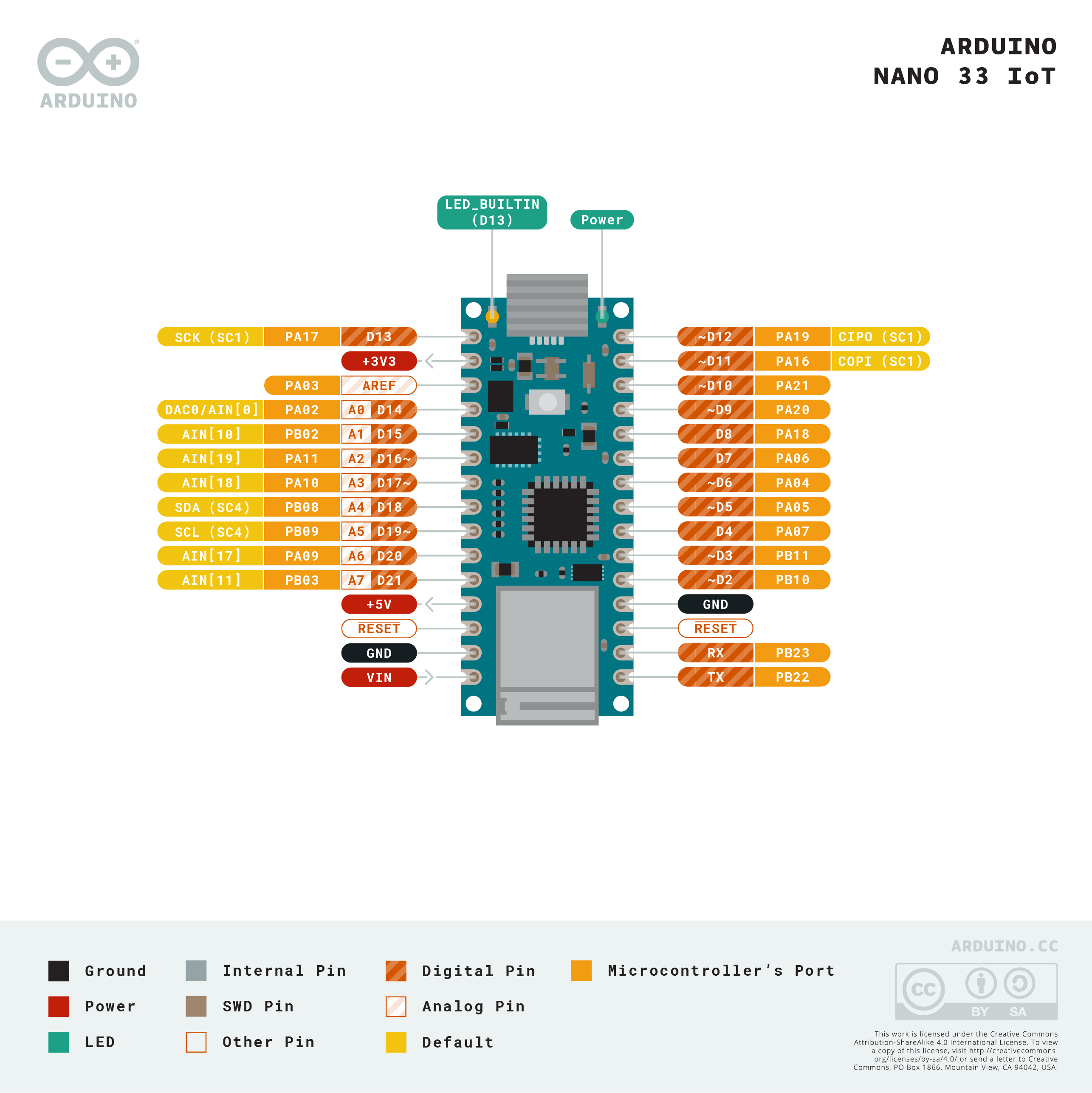
The physical pin numbering for DIP devices goes in a U shape. Holding the micro USB connector at the top, the numbering starts with physical pin 1 on the upper left, counting down the left side to pin 14 on the lower left, then counting from pin 15 on the lower right, to pin 28 on the upper right. For the most part, the left side of the board is power and analog inputs, and the right side is digital I/O pins.
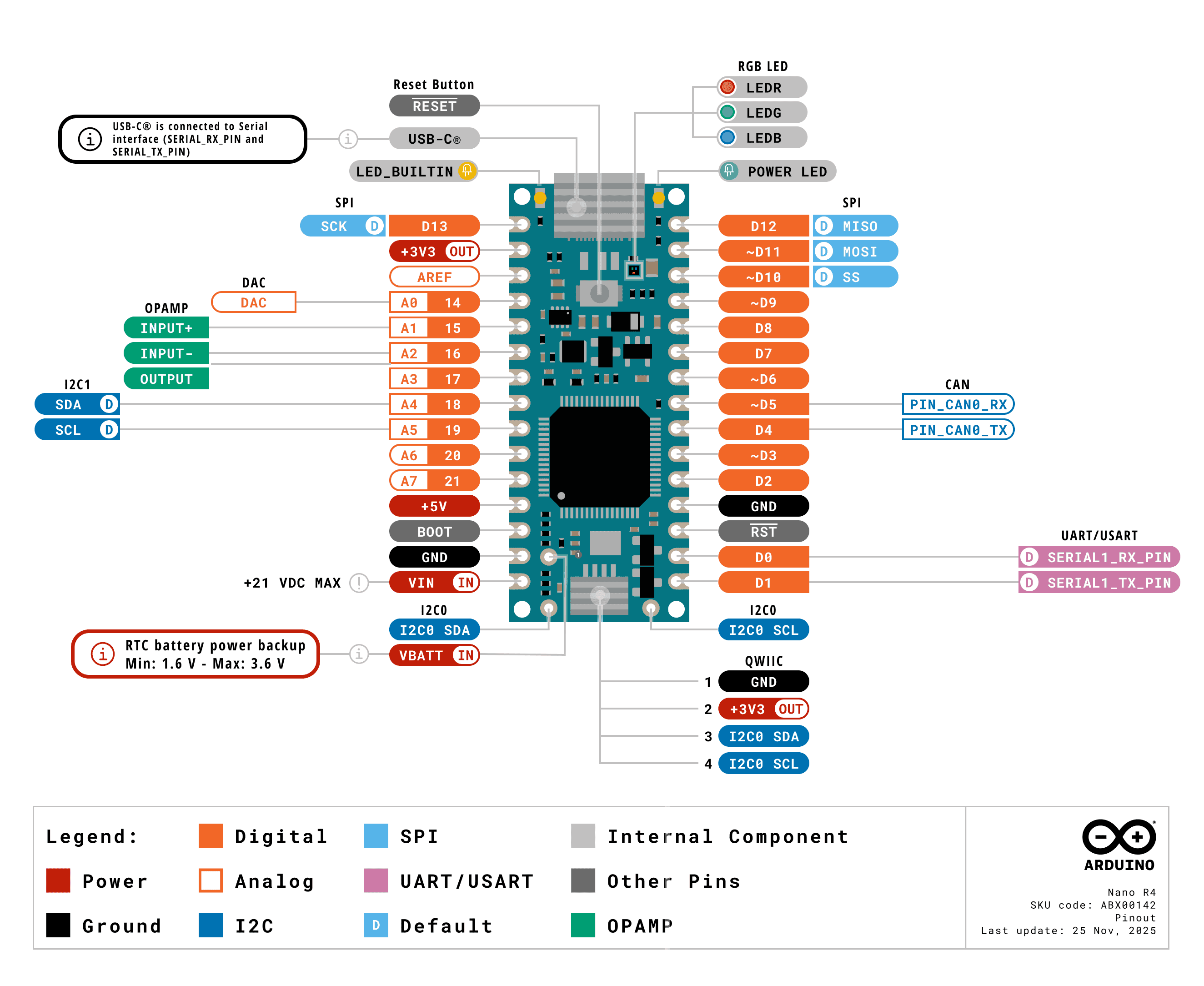
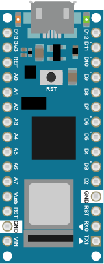
The Nano boards all follow a similar pin layout, as follows, counting from physical pin 1 (upper left) to pin 15 (lower left) across to pin 16 (lower right) to pin 30 (upper right). Figure 1 shows the pin diagram.
Pin 1: Digital I/O 13
Pin 2: 3.3V output
Pin 3: Analog Reference
Pin 4-11: Analog in A0-A7; Digital I/O 14-21 Pin 12: +5V
The full specifications of the Nano R4 and an official pin diagram can be found on its User Manual page.
Typical Breadboard Layout
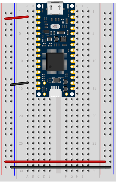
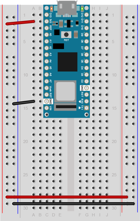
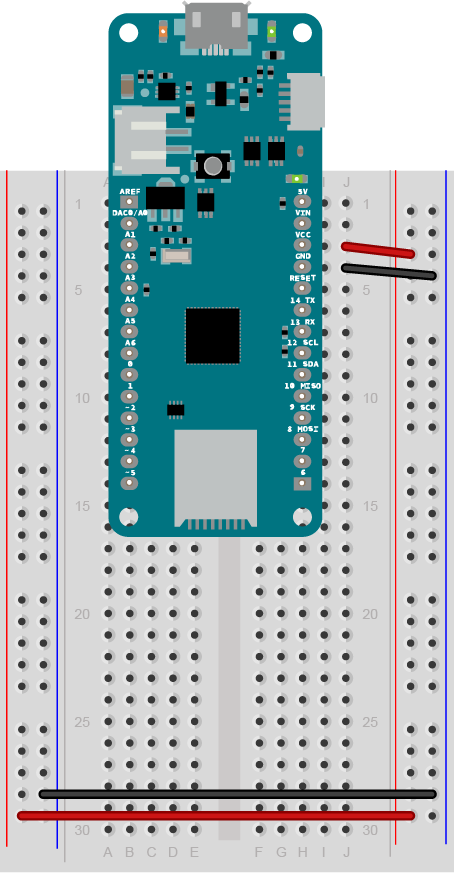
Figure 2. Breadboard view of an Arduino Nano R4 connected to a breadboard.
In a typical breadboard layout for the Nano R4, The +3.3 volts and ground pins of the Nano are connected by red and black wires, respectively, to the left side rows of the breadboard. +3.3 volts is connected to the left outer side row (the voltage bus) and ground is connected to the left inner side row (the ground bus). The side rows on the left are connected to the side rows on the right using red and black wires, respectively, creating a voltage bus and a ground bus on both sides of the board. If you are making a 5-volt circuit instead of a 3.3-volt circuit, you can use the +5 volt pin (pin 12) instead of the +3.3 volt pin.
Like many microcontrollers these days, the Nano R4 uses a USB-C connector. This is a delicate connector, and you shouldn’t handle the board by the connector. If you are mounting the board in a project box or as a wearable and you are using the USB connection, make sure the cable and the board are mounted so that they won’t move relative to each other.
I2C and the Qwiic Connector
The Nano R4 has two I2C buses. The first I2C bus on pins A4 and A5 operates at +5V, like the Nano R4 itself. This bus can be connected to using the Wire library, as usual. The second I2C bus is connected to the qwiic connector, and operates on +3.3V.
The Qwiic connector, the small rectangular part at the bottom center, gives you an easy way to connect I2C peripherals to your board using Qwiic or Qwiic-compatible connectors. Sparkfun’s Qwiic sensors, Adafruit’s Stemma sensors, and Arduino’s Modulino sensors are all compatible. For more on these, see this section of the I2C introduction. For an example, see this lab on the Sparkfun Qwiic Shield for Nano.
Processor
The Nano 33 IoT has a Renesas R7FA4M1AB3CFM 32-bit processor. It’s considerably faster than the Uno’s processor (48MHz clock speed compared to the Uno’s 16MHz, and a 32-bit processor compared to the Uno’s 8-bit processor) and has more memory (256 kB flash, 32 kB SRAM and 8 kB data memory (EEPROM) compared to the Uno’s 2KB/32KB). That makes for more programming space at a faster speed.
Input and Output (GPIO) Pins
The Nano R4 has 14 digital I/O pins and 8 analog input pins. The analog in pins can also be used for digital in and out, for a total of 22 digital I/O pins. Of those, 6 can be used for PWM out (pseudo-analog out): digital pins 3, 5, 6, 9, 10, and 11. One pin A0, can also be used as a true analog out, because it has a digital-to-analog converter (DAC) attached (here’s an example of how to use it). There are also more hardware interrupt pins than the Uno; pins 0,1,2,3,8,8,12,13, and A1 through A6 can be used as hardware interrupts. Hardware interrupts make it possible to read very fast changes in digital input and output. For example, rotary encoders work best when attached to interrupt pins.
Serial and USB
The Nano 33 IoT is USB-native. That means it can operate as a few different USB devices: asynchronous serial, keyboard or mouse (also known as Human Interface Device, or HID). This is different than the Uno, which has a dedicated USB-to-serial chip on the board, but can only operate as a USB serial device.
There’s also a second asynchronous serial port on pins 0 and 1 that you can use for connecting to other serial devices while still connecting to your personal compuuter. The serial port on pins 0 and 1 is called Serial1, so you’d type Serial1.begin(9600) to initialize it, for example.
Real-Time Clock
The Nano R4 also has a real-time clock module built into the processor, which is accessible using the RTC library that also works on the Uno R4. With this, you can keep track of hours, minutes and seconds much easier. As long as the board is powered, the realtime clock will keep time. Like all libraries, it comes with examples when you install it.
Scheduler
The Nano 33 IoT can run multiple loops at once, using the Scheduler library. When you’ve got an application that needs two or more independent loop functions, this can be a quick way to do it.
Uploading to the Nano R4
If you’ve used an Uno before, and are migrating to the Nano R4 board, you may notice that the serial connection behaves differently. When you reset the MKR, Nano, or Leonardo boards, or upload code to them, the serial port seems to disappear and re-appear. The newer boards can communicate natively using USB, unlike the Uno R3. They don’t need a separate USB-to-serial chip. Because of this, they can be programmed to operate as a mouse, or as a keyboard. Since they are USB-native, their USB connection gets reset when you upload new code or reset the processor. That’s normal behavior for them; it’s as if you turned off the device, then turned it back on. Once it’s reset, it will let your computer’s operating system know that it’s ready for action, and your serial port will reappear. This takes a few seconds. It means you can’t reset the board and then open the serial port in the next second. You have to wait those few seconds until the Arduino board has made itself visible to the computer’s operating system again.
If you’re doing keyboard or mouse, the serial port number will also change when you add those functions. You’ll still be able to send and receive serial data as usual, but you’ll have to re-choose the port in the Boards -> Port submenu after you program your Nano to be a HID device.
If you have trouble getting the Nano R4 to appear in the Arduino IDE, double-tap the reset button at the top center of the board. This will put the board into bootloader mode, meaning that it will show up as a serial device, but not start running the sketch yet. This mode also makes it easier to recover your board if you write a sketch you can’t control, such as a runaway mouse sketch.
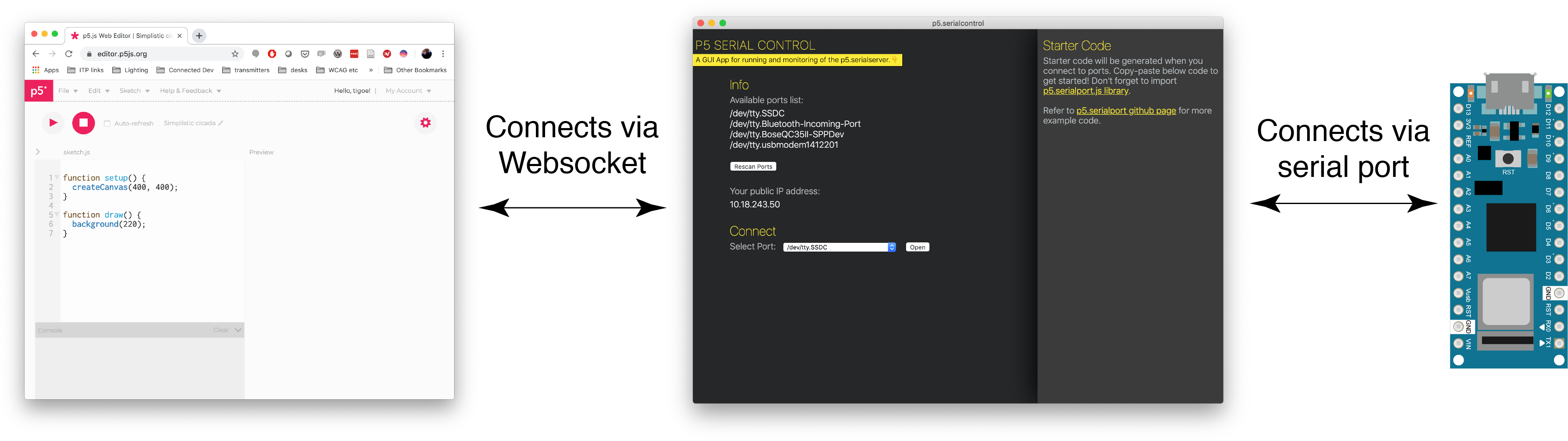
Asynchronous serial communication is not part of the core of p5.js, nor is it part of the core for web browsers. To read serial in a p5.js sketch, or in a web page in general, you need some help. One approach is to open a separate application that connects to the serial port and offers a webSocket connection to the browser. This is the approach that the p5.serialport library and the p5.serialcontrol app take. Another approach is to use the browser API called WebSerial. This is the approach that the p5.webserial library takes.
The difference between them is best illustrated by Figures 1 and 2 below. With p5.seriaport, you must open another application on your computer, p5.serialcontrol, to communicate with the serial port. It is this application that handles serial communication, not the p5.js sketch in the browser. This can be more complicated for beginning users.
Figure 1. Diagram of the connection from the serial port to p5.js through p5.serialcontrol
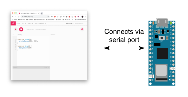
Figure 2. Diagram of the connection from the serial port to p5.js through p5.webserial
p5.serialport/p5.serialcontrol:
p5.webserial:
advantages: * works in all browsers. * Allows your browser to connect to the serial port of a remote computer, if that computer is running a web server program. * Supports opening multiple serial ports at the same time
advantages: * connection is direct to the browser, making it easier for beginners to learn
disadvantages: * requires a third application (p5.serialcontrol), making it more difficult for beginners to learn
disadvantages: * only works in Chrome and Edge browsers * No connection to remote computers * Not sure if it supports a second serial port.
Table 1. Comparing p5.seriaport to p5.webserial
The APIs of p5.serialport and p5.webserial are similar, so it’s pretty straightforward to convert between them.
The code below is a typical p5.serialport setup. You make an instance of the p5.serialport library with the port name, then you make callback functions for the primary tasks:
let serial;          // variable to hold an instance of the serialport library
let portName = '/dev/cu.usbmodem1421';  // fill in your serial port name here

function setup() {
  serial = new p5.SerialPort();       // make a new instance of the serialport library
  serial.on('list', printList);  // set a callback function for the serialport list event
  serial.on('connected', serverConnected); // callback for connecting to the server
  serial.on('open', portOpen);        // callback for the port opening
  serial.on('data', serialEvent);     // callback for when new data arrives
  serial.on('error', serialError);    // callback for errors
  serial.on('close', portClose);      // callback for the port closing

  serial.list();                      // list the serial ports
  serial.open(portName);              // open a serial port
}
The code below is a typical p5.webserial setup. You check t see if WebSerial is available, and then you make an instance of the p5.webserial library, then you look for ports using getPorts():
// variable to hold an instance of the p5.webserial library:
const serial = new p5.WebSerial();
 // port chooser button:
let portButton;
// variable for incoming serial data:
let inData;

function setup() {
   // check to see if serial is available:
   if (!navigator.serial) {
    alert("WebSerial is not supported in this browser. Try Chrome or MS Edge.");
  }
  // check for any ports that are available:
  serial.getPorts();
  // setup function continues below:
Unlike with p5.serialport, you don’t pass in the port name. Instead, the user chooses the port with a pop-up menu:
  // if there's no port chosen, choose one:
  serial.on("noport", makePortButton);
  // open whatever port is available:
  serial.on("portavailable", openPort);
  // setup function continues below:
Then you make callback functions for the primary tasks. These are similar to p5.serialport’s callbacks:
   // handle serial errors:
  serial.on("requesterror", portError);
  // handle any incoming serial data:
  serial.on("data", serialEvent);
  serial.on("close", makePortButton)
  // setup function continues below:
You also add listeners for when the USB serial port enumerates or de-enumerates. This way, if you unplug your serial device or reset it, your program automatically reopens it when it’s available:
  // add serial connect/disconnect listeners from WebSerial API:
  navigator.serial.addEventListener("connect", portConnect);
  navigator.serial.addEventListener("disconnect", portDisconnect);
} // end of setup function
The functions in each API are similar too:
p5.serialport functions (from the library’s guide)
read() returns a single byte of data (first in the buffer)
read() — reads a single byte from the queue (returns a number)
readChar() returns a single char, e,g, ‘A’, ‘a’
readChar() — reads a single byte from the queue as a character (returns a string)
readBytes() returns all of the data available as an array of bytes
readBytes() — reads all data currently available in the queue as a Uint8Array.
readBytesUntil(charToFind) returns all of the data available until charToFind is encountered
readBytesUntil(charToFind) — reads bytes until a character is found (returns a Uint8Array)
readString() returns all of the data available as a string
readStringUntil(charToFind) returns all of the data available as a string until charToFind is encountered
readStringUntil(stringToFind) — reads out a string until a certain substring is found (returns a string)
last() returns the last byte of data from the buffer
lastChar() returns the last byte of data from the buffer as a char
readLine() — read a string until a line ending is found (returns a string)
write() – sends most any JS data type out the port.
write() – sends most any JS data type out the port.
print()– sends string data out the serial port
println() – sends string data out the serial port, along with a newline character.
Table 2. Comparison of p5.serialport and p5.webserial APIs
Both p5.serialport and p5.webserial will do the job of getting bytes from a serial device like an Arduino or other microcontroller to p5.js and vice versa. Which you use depends on what you need. p5.webserial is great if you’re connected directly to the browser’s computer via USB. For most serial applications, this is the way to go. Alternately, p5.serialport offers the advantage that you can run p5.serialcontrol app on your browser’s computer or on another computer on the same network. That way, a browser on your phone or tablet can communicate to the serial device via the computer running p5.serialcontrol.
Distance sensors can be used for any number of applications including range finding, user detection, and obstacle avoidance. Distance sensors are increasingly commonplace in automobiles to facilitate parking and provide enhanced situational awareness. They are used in smartphones to prevent unintended touchscreen activation when holding the device to your ear, and they are integral to touch free paper towel dispensers. Any camera with autofocus relies on a distance sensor. Whether stationary or in motion, distance sensors take readings using one of three methods: signal strength (how diminished is the emitted signal when reflected off a target); triangulation (distance as a function of the angle at which the emitted signal is reflected off the target); or time of flight (the time it takes for a signal to be emitted, reflected off the target, and received). In this lesson, you’ll learn a few principles of working with these sensors, and see some examples.
What You’ll Need to Know
To get the most out of this page, it helps to be familiar with the following concepts:
It’s important to understand what distance sensors can do, and what they can’t do. Two common uses for distances sensor are measuring distance, or how far away from the sensor a person or object is, and detecting presence, or whether there is a person in front of the sensor at all. Many distance sensors use the term proximity to refer to presence as well. A third use that many people often want from these sensors is to detect attention. Distance and presence or proximity are easy to sense. Attention is a more complex problem, not solved by distance sensors alone. To know whether a sensor can do the job at all, you should also know about where it can sense objects or people. The terms Field of View or Angle of View are often used to describe this in technical documents.
Measuring Distance vs Detecting Presence
“Most sensors that read the distance from a target send out some form of energy (light, magnetism, or sound). They measure the amount of energy that reflects off the target and compare it with the energy that went out. Then they convert the difference into an electrical voltage or digital signal that you can read on a microcontroller… This principle is common to many different sensors and across many scales. On a small scale, domestic robots such as Roombas emit an infrared light and wait for the reflected IR light from an obstacle to navigate a room. On a large scale, airplane radar systems operate by sending out a radio signal and measuring the time it takes for the signal to bounce back from a target….
“One common use for distance sensors is to track a person moving in front of an object in order to trigger the object to action when the person gets close enough. This can be very effective, but keep in mind that being present and paying attention are not the same thing, as any parent or teacher can confirm. Imagine that you want to sense when a person is looking at your painting so that you can make the painting respond in some way. You could put a ranging sensor in front of the painting and look for a person to get close enough, but this sensor alone won’t tell you whether she’s got her back to the painting or not. Sensing attention is a more complex problem.”
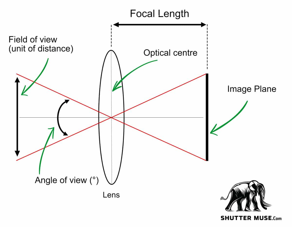
You’ll often see one of two terms referring to a distance sensor’s capabilities: Angle of View or Field of View. While the term “Angle of View” is more accurate, you’ll most often see “Field of View” in documentation for these sensors. Angle of View describes the shape of the cone projected from the sensor within which a signal is either emitted or received and its value is measured in degrees. True Field of View describes the plane perpendicular to the sensor at any given distance that is bounded by the Angle of View. Note that a sensor’s emitter and receiver may have different Angles of View but they are designed to overlap to the greatest extent possible. Figure 1 illustrates the relationship between angle of view and field of view.
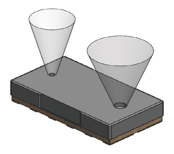
Figure 2 shows a typical distance sensor’s two main elements, the emitter and the receiver, showing the the angle of transmission from the transmitter and angle of view from the receiver. They sit beside each other on the device, pointing the same direction.
Whether you’re dealing with an IR proximity sensor, LiDAR distance sensor, or time of flight sensor, there are a few features you’ll need to consider:
Range – Distance sensors come with different minimum and maximum ranges.
Resolution – How granular the units of measurement. Not to be confused with a sensor’s accuracy.
Field of View – More accurately described as Angle of View when measured in degrees, the Field of View describes the area in which a target will trigger a reading at a given distance from the sensor.
Susceptivity to ambient light conditions – With the exception of ultrasonic sensors, the presence of ambient light will affect a distance sensor’s performance. Direct light is more disruptive than indirect, outdoor light more so than indoor, and incandescent light sources more so than artificial.
Some target properties will affect the sensor’s response. For example, large faceted shapes or concave shapes (like the inside of a bowl, or a hat) might not reflect the beam back to the sensor well. Other factors which could affect the response include:
size
orientation (wrt the sensor)
color
transparency
reflectance
texture
Electrical Characteristics – As with any electronic sensor, you should pay attention to current consumption and make sure the rated voltage of your distance sensor is compatible with your microprocessor.
Interface – Distance sensors come with a variety of interfaces. Some provide a changing analog voltage based on range. Others will provide a UART asynchronous or an I2C synchronous serial interface. Ultrasonic distance sensors will provide a changing pulse width that corresponds with the changing properties of the sensor. Nowadays, most light-based distance sensors are I2C.
Extra Features – in addition to the basic physical properties, some distance sensors will have additional features, like the ability to measure ambient light, rudimentary gesture detection, or sophisticated control features like the ability to set angle of view or specific regions of interest (ROI).
Most vendors of sensor modules do not actually make the sensors themselves, they just put them on a breakout board along with the reference circuit, for convenience. While you might buy your distance sensor from Sparkfun, Adafruit, Seeed Studio, or Pololu, for example, the chances are the actual sensor is manufactured by another company like AMS, Sharp, ST Microelectronics, or Vishay. When you shop for a sensor module, check out the manufacturer’s datasheet in addition to the vendor’s tech specs. It’s also worth doing a comparison search with the sensor part number on Octopart.com to see who else might make a breakout board.
Ultrasonic Distance Sensors
Ultrasonic distance sensors use a transducer to emit a pulse of ultrasound at 40 MHz measuring the time it takes for the pulse to bounce off the target and return to the sensor and calculating distance based on the speed of sound. Although it’s unusual to see them described as such, technically they are a sonic time-of-flight sensor. Ultrasonic distance sensors are immune to ambient lighting conditions and target transparency however because sound transmission is influenced by the physical properties of air, accuracy is affected by ambient sound, temperature, and humidity. A ‘soft’ sound absorbing target with a surface covered by cloth will impact accuracy, as will a target with an irregular surface.
HC-SR04 distance sensors are a staple of many starter kits built around the Arduino Uno, which means they are not plug-and-play compatible with 3.3V Arduino boards like the Nano 33 IoT. It’s simple enough to incorporate a voltage divider into your circuit, however, and if you’re feeling adventurous, the HC-SR04 can be permanently modified for use with either 3.3V or 5V logic.
The simplest approach to measuring distance using infrared light is to measure the amount of emitted IR light that bounces off a target and reflects back to the sensor. The ranges are relatively small — between 0 and 20cm — and the language used is ‘proximity’ rather than ‘distance’.
Some optical time-of-flight distance sensors are based on IR LED emitters. They can be pricey. The Benewake TFmini sold by Adafruit, SparkFun and Seeed is capable of ranging distances up to 12 meters and while it requires 5V to operate, it uses 3.3V logic to communicate. Unlike other distance sensors that use I2C, the TFmini uses the UART protocol for asynchronous serial communication.
The Garmin LIDAR-Lite V4 — available at Adafruit and SparkFun (also available with Qwiic connector) — has a 10 meter range and is more expensive than the Benewake sensor but comes with some additional features including I2C serial protocol and wireless control using Garmin’s open ANT Protocol, a low power wireless protocol alternative to BLE.
Note that both Benewake and Garmin take creative license and, while not technically accurate, nonetheless market the two products above as ‘LiDAR’ distance sensors.
Infrared LED Triangulation Sensors
Another method for calculating distance using infrared light is triangulation. A pulse of IR light is emitted and range is determined based on the angle of reflection. Most of the maker / hobbyist sensors of this category are manufactured by Sharp. They come in both analog and digital output variations but because most of them require 5V, they can be used with the Uno but not the Nano 33 IoT. The Sharp GP2Y0A60SZLF is an exception, operating at 3V. Pololu makes a breadboard-friendly module with this sensor.
Maximum distances for analog output sensors range from 5cm to 80cm depending on the model. For sensors with digital output, maximum distances range from 1.5cm to 550cm.
LiDAR Distance Sensors
LiDAR distance ranging sensors like the Garmin LIDAR-Lite v3 available from Adafruit and SparkFun use time-of-flight to calculate distance as a function of the time it takes a pulse of emitted laser light to reflect off a target and return to the sensor. The Garmin LIDAR-Lite v3 is capable of very rapid readings measuring distances up to 40 meters although at a resolution of centimeters rather than millimeters. Data can be sent to the microprocessor as either a digital signal using I2C or an analog signal using pulse width modulation. Distance sensors of this kind are often used in robotics and autonomous vehicles; they are quite expensive and less likely to be of practical use to PComp projects.
LiDAR is an acronym for light detection and ranging pr laser imaging, detection, and ranging. Note that some distance sensors marketed as LiDAR are actually lensed IR LED time-of-flight sensors and do not actually user lasers.
Another example of optical time-of-flight, these distance sensors combine a vertical cavity surface emitting laser (VCSEL) with a single-photon avalanche diode (SPAD) array to measure the time it takes a photon of light to travel from the sensor, to the target, and back. Distance is then calculated using the speed of light, which is a constant. VCSEL distance sensors provide true laser-based ranging with high resolution (millimeters rather than centimeters) in a very small form factor. ST’s VL53L0X and ST’s VL53L1X are VCSEL sensors. A lab exercise on the VL53L0x sensor can be found on this site.
RADAR
RADAR is an acronym for Radio Detection and Ranging. Radar is a technology that dates back to the 1940’s. Despite being a mature technology, though, it is still not as inexpensive or as ubiquitous as other forms of distance ranging. Seeed Studio makes a Doppler Radar module, however, for those interested in radar: Seeed Grove Doppler Radar
What To Look For in a Distance Sensor Library
Different vendors will often write their own libraries for the distance sensors they sell. When you’re looking at a given vendor’s product, take a look at the properties of the sensor in the vendor’s datasheet, and the list of public functions in the library’s API. Does the library give you the functions of the sensor that you need? If the sensor supports multiple sensing ranges, does the library give you access to setting and getting the range? Is it well-documented, and well-commented? Are there simple, clear, well-commented examples?
For example, both SparkFun and Pololu make breakout boards for the VL53L1X Time-of-Flight sensor. The VL53L1X is typical of a next gen distance sensor; it’s got an I2C interface, operates at 2.8V, and offers a large range from 4cm to 400cm. The SparkFun hookup guide is more accessible than the Using the VL53L1X section on Pololu’s product page but neither provides a summary of all the functions in their libraries. To see that, you need to look at the header files for each library.
Pololu offers two different libraries for the VL53L1X. The Pololu VL53L1X library is streamlined to use less resources but doesn’t surface some of the more technical features of the sensor. On the other hand, the Pololu ST VL53L1X API library is a largely literal implementation of ST’s VL53L1X Full API, providing more advanced functionality at the expense of a larger memory footprint and a more opaque code base divided into multiple header files geared less toward the student or hobbyist than someone with an electrical engineering background.
By comparison, SparkFun’s header file is less verbose and significantly shorter than either of the Pololu offerings with clean, succinct, in-line comments that make it accessible and easy to navigate. The public functions start around line 35. Both are functional libraries, though, and you should choose based on the features you want and how easy you find each to use.
You can find further notes on how to pick a library in this lab exercise for the APDS-9960 Color, Light, and Gesture sensor.
Conclusion
There are dozens of distance sensors on the market, and as they become more ubiquitous in electronic devices, they continue to get smaller, cheaper, more sophisticated and more power-efficient. The principles laid out here should give you a basis for assessing new sensors as needed.
The Arduino Nano 33 IoT is a useful little microcontroller board. It can do the things that the Arduino Uno can, and it has a number of additional features for physical computing projects. In 2019, we started using it as the standard for Intro to Physical Computing. This page introduces some of the functions that this board supports.
Form Factor
The Nano 33 IoT is based on the original Arduino Nano pin layout, so if you’ve used the Nano in past projects, the layout is the same. It’s a dual-inline package (DIP) format, meaning it’s got two rows of pins spaced 0.1 inches apart, so it fits nicely on a solderless breadboard. You can get it with or without header pins, and it’s small enough that you can incorporate it in handheld projects as well.
The physical pin numbering for DIP devices goes in a U shape. Holding the micro USB connector at the top, the numbering starts with physical pin 1 on the upper left, counting down the left side to pin 14 on the lower left, then counting from pin 15 on the lower right, to pin 28 on the upper right. For the most part, the left side of the board is power and analog inputs, and the right side is digital I/O pins.
In brief, the Nano pins are as follows, counting from physical pin 1 (upper left) to pin 15 (lower left) across to pin 16 (lower right) to pin 30 (upper right):
Pin 1: Digital I/O 13
Pin 2: 3.3V output
Pin 3: Analog Reference
Pin 4-11: Analog in A0-A7; Digital I/O 14-21 Pin 12: VUSB (not normally connected)
Pin 13: Reset
Pin 14: Ground
Pin 15:Vin
Pin 16: Digital I/O pin 1; Serial1 UART TX
Pin 17: Digital I/O pin 0; Serial1 UART RX
Pin 18: Reset
Pin 19: Ground
Pin 20-30: Digital I/O pins 2-12
Figure 1. Drawing of the Nano 33 IoT
The microcontroller pin functions page details the functions of each pin for the Nano and other Arduino boards. The full specifications of the Nano 33 IoT and an official pin diagram can be found on its Getting Started page.
Typical Breadboard Layout
Figure 2. Breadboard view of an Arduino Nano connected to a breadboard.
In a typical breadboard layout, The +3.3 volts and ground pins of the Nano are connected by red and black wires, respectively, to the left side rows of the breadboard. +3.3 volts is connected to the left outer side row (the voltage bus) and ground is connected to the left inner side row (the ground bus). The side rows on the left are connected to the side rows on the right using red and black wires, respectively, creating a voltage bus and a ground bus on both sides of the board.Other board layouts can be found on the Breadboard Layouts page.
Handling the Board
You should be careful when handling the Nano 33 IoT as there are two delicate parts on it: the MicroUSB connector at the top, and the WiFi/Bluetooth antenna at the bottom. Figure 2 shows a picture of the board.
Like many microcontrollers these days, the Nano 33 IoT uses a MicroUSB connector. This is a delicate connector, and you shouldn’t handle the board by the connector. If you are mounting the board in a project box or as a wearable and you are using the USB connection, make sure the cable and the board are mounted so that they won’t move relative to each other.
The WiFi/Bluetooth Antenna is the small rectangular part at the bottom center. If it is broken off, your WiFi and Bluetooth range will be significantly reduced. For more on caring for it, see the Care of your Nano 33 IoT video and Breadboard Basics.
Figure 2. Arduino Nano 33 IoT
Power
The Nano 33’s first difference from the Uno is that it operates on 3.3 volts instead of 5 volts. This might be an issue for some older sensors or actuators, but most modern ones will operate on 3.3V. For most projects, you’ll supply 3.3V from the Nano’s +3V3 pin (physical pin 2) and ground from one of the ground pins (physical pins 13 or 18).
If you’re powering the Nano 33 IoT from USB, then the Vin pin (physical pin 14) will supply 5V from the USB connection. You can also supply power the Nano 33 IoT on this pin, up to 21V. If power is fed through this pin, the USB power source is disconnected. If you need 5V power when you’re powered via the Vin pin, you can solder the VUSB jumper on the back, behind pin 19. When you do this, then the VUSB pin will supply 5V whenever the board is powered via the Vin pin.
Processor
The Nano 33 IoT has an ARM Cortex-M0 32-bit SAMD21 processor. It’s considerably faster than the Uno’s processor (48MHz clock speed compared to the Uno’s 16MHz, and a 32-bit processor compared to the Uno’s 8-bit processor) and has more memory (32KB SRAM/256KB flash compared to the Uno’s 2KB/32KB). That makes for more programming space at a faster speed.
Uploading to the Nano 33 IoT
If you’ve used an Uno before, and are migrating to the Nano board, you may notice that the serial connection behaves differently. When you reset the MKR, Nano, or Leonardo boards, or upload code to them, the serial port seems to disappear and re-appear. Here’s why:
There is a difference between the Uno and most of the newer boards like the MKR boards, the Nano 33 IoT and BLE, the Leonardo: the Uno has a USB-to-serial chip on the board which is separate from the microcontroller that you’re programming. The Uno’s processor, an ATMega328, cannot communicate natively via USB, so it needs the separate processor. That USB-to-serial chip is not reset when you upload a new sketch, so the port appears to be there all the time, even when your Uno is being reset.
The newer boards can communicate natively using USB. They don’t need a separate USB-to-serial chip. Because of this, they can be programmed to operate as a mouse, as a keyboard, or as a USB MIDI device. Since they are USB-native, their USB connection gets reset when you upload new code or reset the processor. That’s normal behavior for them; it’s as if you turned off the device, then turned it back on. Once it’s reset, it will let your computer’s operating system know that it’s ready for action, and your serial port will reappear. This takes a few seconds. It means you can’t reset the board and then open the serial port in the next second. You have to wait those few seconds until the Arduino board has made itself visible to the computer’s operating system again.
If you’re doing MIDI or keyboard or mouse, the serial port number will also change when you add those functions. You’ll still be able to send and receive serial data as usual, but you’ll have to re-choose the port in the Boards -> Port submenu after you program your Nano to be a MIDI or HID device.
If you have trouble getting the Nano 33 IoT to appear in the Arduino IDE, double-tap the reset button at the top center of the board. This will put the board into bootloader mode, meaning that it will show up as a serial device, but not start running the sketch yet. This mode also makes it easier to recover your board if you write a sketch you can’t control, such as a runaway mouse sketch.
Input and Output (GPIO) Pins
The Nano 33 IoT’s got 14 digital I/O pins and 8 analog input pins. The analog in pins can also be used for digital in and out, for a total of 22 digital I/O pins. Of those, 11 can be used for PWM out (pseudo-analog out): digital pins 2, 3, 5, 6, 9, 10, 11, 12, A2, A3, and A5. One pin A0, can also be used as a true analog out, because it has a digital-to-analog converter (DAC) attached (here’s an example of how to use it). There are also more hardware interrupt pins than the Uno; pins 2, 3, 9, 10, 11, 13, A1, A5, and A7 can be used as hardware interrupts. Hardware interrupts make it possible to read very fast changes in digital input and output. For example, rotary encoders work best when attached to interrupt pins.
Serial and USB
The Nano 33 IoT is USB-native. That means it can operate as a few different USB devices: asynchronous serial, keyboard or mouse (also known as Human Interface Device, or HID), and USB MIDI. This is different than the Uno, which has a dedicated USB-to-serial chip on the board, but can only operate as a USB serial device.
There’s also a second asynchronous serial port on pins 0 and 1 that you can use for connecting to other serial devices while still connecting to your personal compuuter. The serial port on pins 0 and 1 is called Serial1, so you’d type Serial1.begin(9600) to initialize it, for example.
Synchronous Serial
Like the other Arduinos, the Nano 33 IoT can communicate via Synchronous serial communications using I2C or SPI. The SPI pins are:
SDI- 12
SDO – 11
SCK – 13
CS – 10
The I2C pins are:
SDA – A4
SCL – A5
Inertial Measurement Unit (IMU)
There is an Inertial Measurement Unit (IMU) on the board, combining a 3-axis accelerometer with a 3-axis gyrometer. This enables gesture-based sensing or tap sensing with no extra hardware. The Arduino_LSM6DS3 library supports this sensor. There are some notes at this link and a lab at this link introducing the IMU.
Real-Time Clock
The Nano 33 IoT also has a real-time clock module built into the processor, which is accessible using the RTCZero library. With this, you can keep track of hours, minutes and seconds much easier. As long as the board is powered, the realtime clock will keep time. Like all libraries, it comes with examples when you install it. You can find several additional examples in this gitHub repository.
WiFi and Bluetooth
WiFi and Bluetooth connectivity are available on the Nano 33 IoT via a low-power 2.4GHz radio. Secure communication is ensured through an on-board crypto chip as well. The WiFiNINA library supports the WiFi on this board, and it’s compatible with the WiFi101 library written for the MKR1000. Any examples written for WiFi101 should be able to run just by changing WiFi101.h to WiFiNINA.h. You can find additional WiFi examples at these links:
The Nano 33 IoT can run multiple loops at once, using the Scheduler library. When you’ve got an application that needs two or more independent loop functions, this can be a quick way to do it.
For more on using the Nano 33 IoT, see the various microcontroller Labs on this site, for example:
Inertial Motion Units (IMUs) are sensors that measure movement in multiple axes. Accelerometers measure a changing acceleration on the sensor. They can be used to measure the tilt of the sensor with respect of the Earth, or the force of a hit. They are common in mobile devices and automobiles. Gyrometers measure changing angular motion. They can be used to measure rotation. Magnetometers measure the magnetic force on a sensor. These are usually used to measure the Earth’s gravitational field in order to determine compass heading. IMUs have become increasingly common in microcontroller projects, to the point where they are built into some microcontroller boards like the Arduino 33 IoT and BLE Sense, and the Arduino 101. In this lesson, you’ll learn a few principles of working with these sensors, and see some examples.
What You’ll Need to Know
To get the most out of this lab, you should be familiar with the following concepts and you should install the Arduino IDE on your computer. You can check how to do so in the links below:
Figures 1-4 below show the parts you’ll need for this exercise. Click on any image for a larger view.
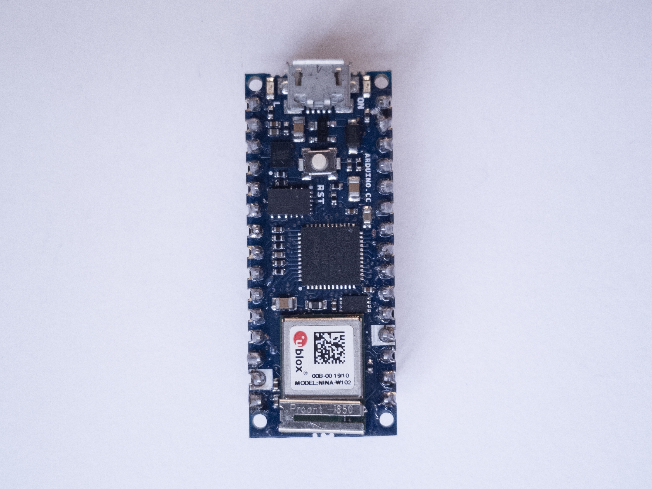
Figure 1. Microcontroller. Shown here is an Arduino Nano 33 IoT. An Uno will do for some of the examples here, though.
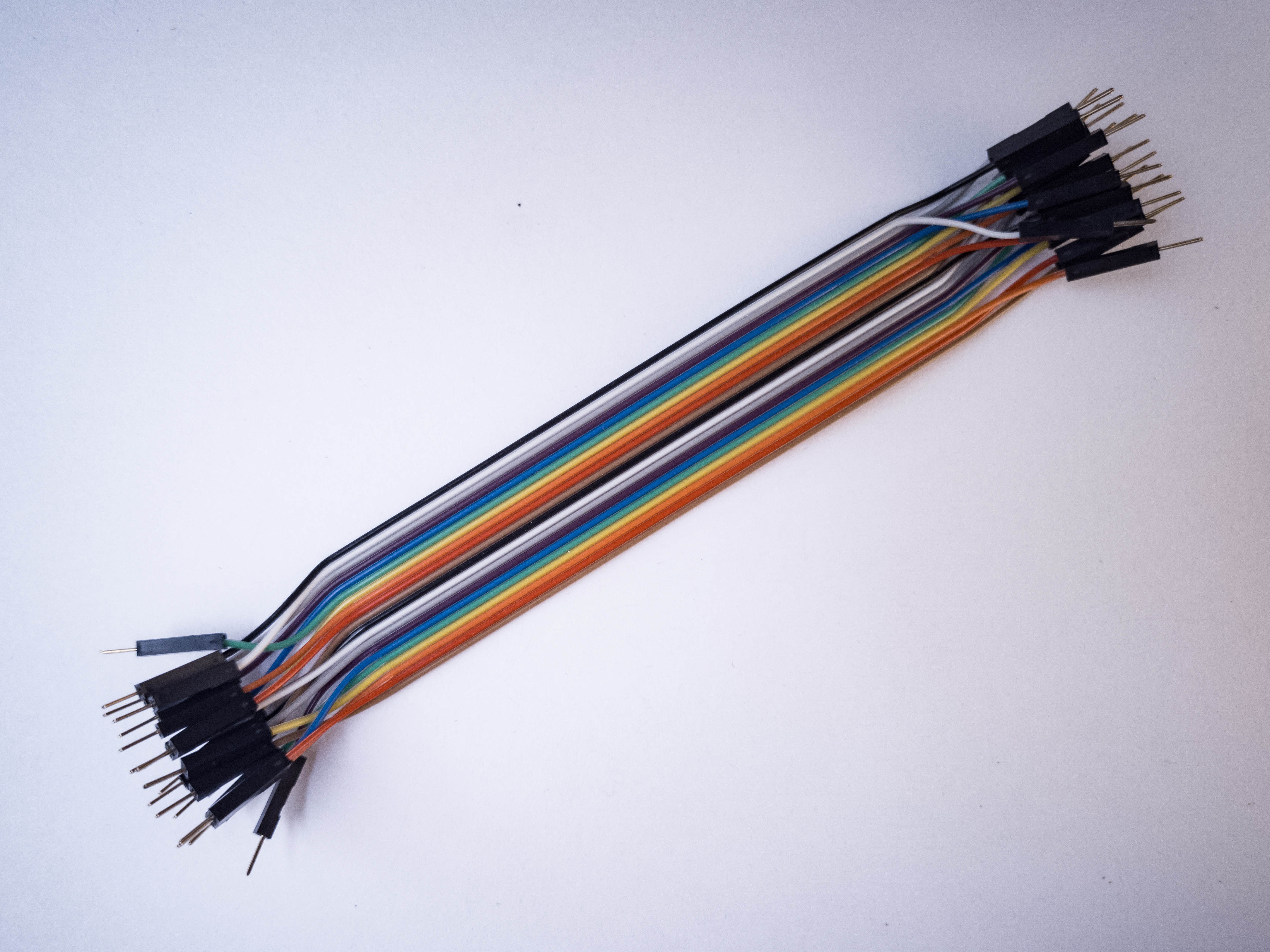
Figure 2. Jumper wires. You can also use pre-cut solid-core jumper wires.
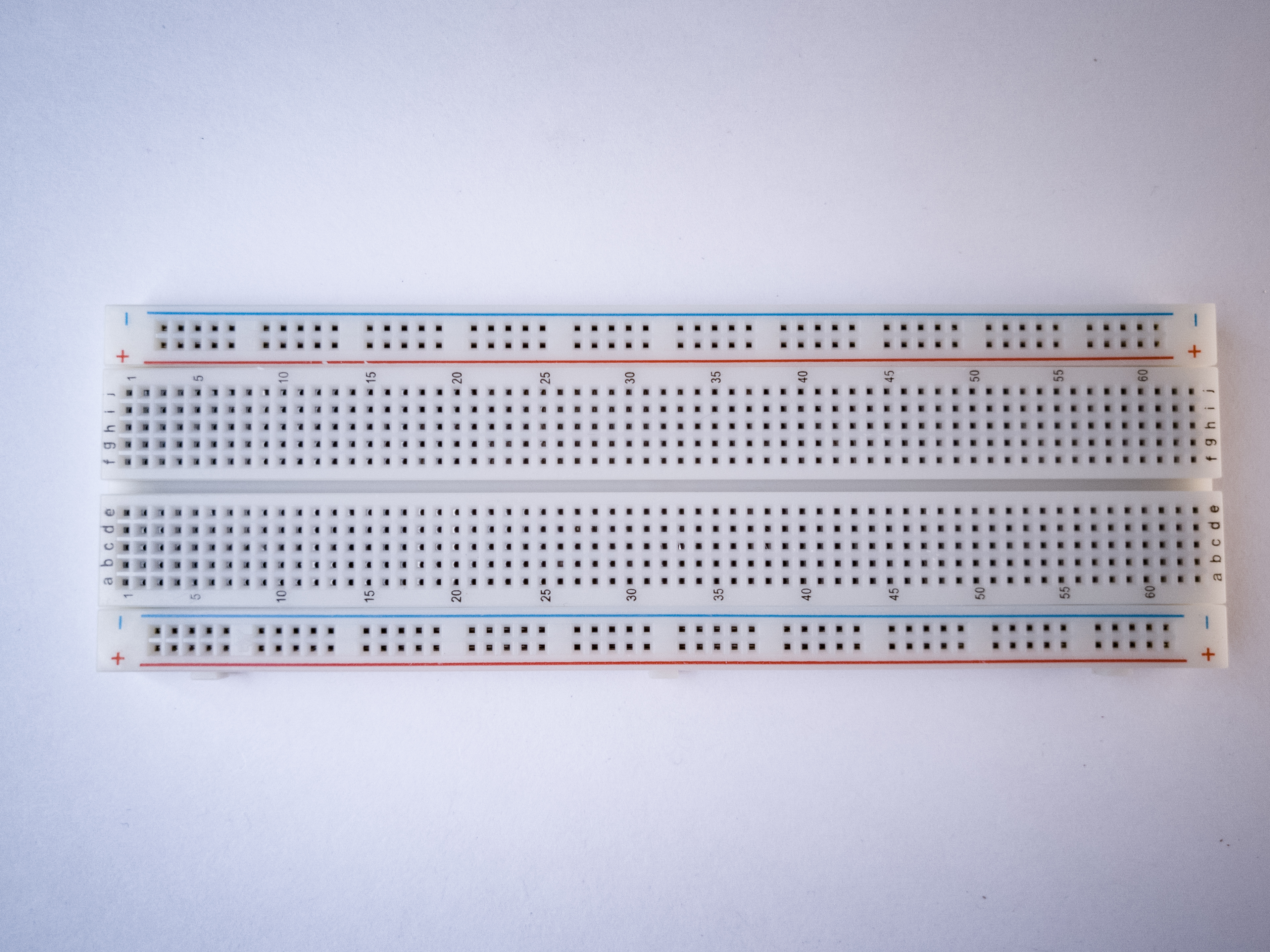
Figure 3. A solderless breadboard
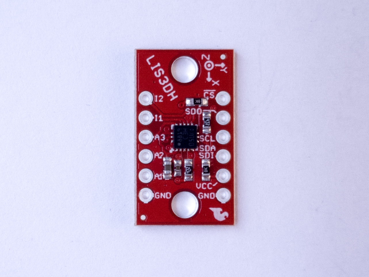
Figure 4. An accelerometer. Shown here is an ST Microelectronics LIS3DH accelerometer. Others will be mentioned below.
Orientation, Position, and Degrees of Freedom
“Orientation, or compass heading, is how you determine your direction if you’re level with the earth. If you’ve ever used an analog compass, you know how important it is to keep the compass level in order to get an accurate reading. If you’re not level, you need to know your tilt relative to the earth as well. In navigational terms, your tilt is called your attitude, and there are two major aspects to it: roll and pitch. Roll refers to how you’re tilted side-to-side. Pitch refers to how you’re tilted front-to-back.
“Pitch and roll are only two of six navigational terms used to refer to movement. Pitch, roll, and yaw refer to angular motion around the X, Y, and Z axes. These are called rotations. Surge, sway, and heave refer to linear motion along those same axes. These are called translations. These are often referred to as six degrees of freedom. Degrees of freedom refer to how many different parameters the sensor is tracking in order to determine your orientation.
“You’ll hear a number of different terms for these sensors. The combination of an accelerometer and gyrometer is sometimes referred to as an inertial measurement unit, or IMU… When an IMU is combined with a magnetometer, the combination is referred to as an attitude and heading reference system, or AHRS. Sometimes they’re also called magnetic, angular rate, and gravity, or MARG, sensors. You’ll also hear them referred to as 6-degree of freedom, or 6-DOF, sensors. There are also 9-DOF sensors that incorporate all three types of sensors. Each axis of measurement is another degree of freedom. [There are] even has 10-DOF sensor[s] that add barometric pressure sensor[s] for determining altitude.”
Whether you’re dealing with an accelerometer, gyrometer, or magentometer, there are a few features you’ll need to consider:
Range – IMU sensors come in different ranges of sensitivity.
Acceleration is generally measured in meters per second squared (m/s^2) or g’s, which are multiples of the acceleration due to gravity. 1g = 9.8 m/s^2. Accelerometers come in ranges from 2g to 250g and beyond. the force of gravity is 1g, but a human punch can be upwards of 100g
Angular motion is measured in degrees per second (dps). Gyro ranges of 125dps to 2000 dps are not uncommon.
Magnetic force is measured in Teslas. In most direction applications, the important measurement, however is the relative magnetic field strength on each axis.
Number of axes – Almost all IMU sensors can sense their respective properties on multiple axes. Whatever activity you’re measuring, you’ll most likely want to know the acceleration, rotational speed, or magnetic force in horizontal and vertical directions. Most sensors give results for the X, Y, and Z axes. Z is typically perpendicular to the Earth, and the other two are parallel to it, but perpendicular to each other.
Electrical Characteristics – as with any electronic sensor, you should pay attention to current consumption and make sure the rated voltage of your IMU is compatible with your microcontroller.
Interface – IMUs come with a variety of interfaces. Some provide a changing analog voltage on each axis. Others will provide an I2C or SPI synchronous serial interface. Older IMUs will provide a changing pulse width that corresponds with the changing properties of the sensor. Nowadays, most IMUs are either I2C, SPI, or analog.
Extra Features – in addition to the basic physical properties, many IMUs will have additional features, like freefall detection or tap detection, or additional control features like the ability to set the sensing rate.
Most vendors of accelerometer modules do not actually make the sensors themselves, they just put them on a breakout board along with the reference circuit, for convenience. While you might buy your IMU from Sparkfun, Adafruit, Seeed Studio, or Pololu, for example, the chances are the actual sensor is manufactured by another company like Analog Devices, ST Microelectronics, or Bosch. When you shop for a sensor module, check out the manufacturer’s datasheet in addition to the vendor’s tech specs.
Analog IMUs
Analog IMU sensors typically have an output pin for each axis that outputs a range from 0 volts to the sensor’s maximum voltage. Most of them only have one form of sensor (accelerometer, gyrometer, magnetometer). Having multiple pins for each type of sensor would be unweildy.
Since it’s possible to have both positive and negative change in a given sensor’s range, the rest value for each output pin is usually in the middle of the voltage range. You need to understand this in order to read the sensor.
Analog Devices’ ADXL series of accelerometers are useful examples of this kind of sensor. There are two similar models, the ADXL335 and the ADXL377. The former is good for simple range of motion applications, and latter is designed for high-acceleration applications, like crashes, punches, and so forth. Both operate at 3.3V. Both output analog voltages for X, Y, and Z. Both output their midrange voltage, about 1.65V, on each axis when it’s at rest (at 0g). The ADXL335 is a +/-3g accelerometer, and the ADXL377 is a +/- 200g accelerometer. While you’d see a significant change on the ADXL335’s axes when you simply tilt the sensor, you’d see barely any when you simply tilt the ADXL377. Why? Consider the math:
The ADXL335 outputs 0V at -3g, 3.3V at +3g, and 1.65V at 0g. That means that 1g of acceleration changes the analog output by 1/6 of its range. If you’re using analogRead() on an Arduino with a 3.3V analog reference voltage, that means you’ve got a range of about 341 points per g of acceleration (1024 / 6). When you tilt the accelerometer to 90 degrees, you’re getting +1g on the X or Y axis. That’s a reading of about 682 using analogRead() on an Arduino. When you tilt it 90 degrees the other way, you’re getting -1g on the same axis, or about 341 using analogRead().
The ADXL377 outputs 0V at -200g, 3.3V at +200g, and 1.65V at 0g. That means 1g of acceleration changes the output by only 1/400 of its range. The same tilting action described above would give you a change from about 510 to 514 using analogRead(),using the same math as above.
This lesson applies whether you’re measuring acceleration, rotation, or magnetic field strength. Make sure to use a sensor that matches the required range otherwise you won’t see much change, particularly with an analog sensor.
Analog Accelerometer Example
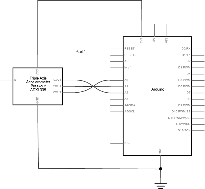
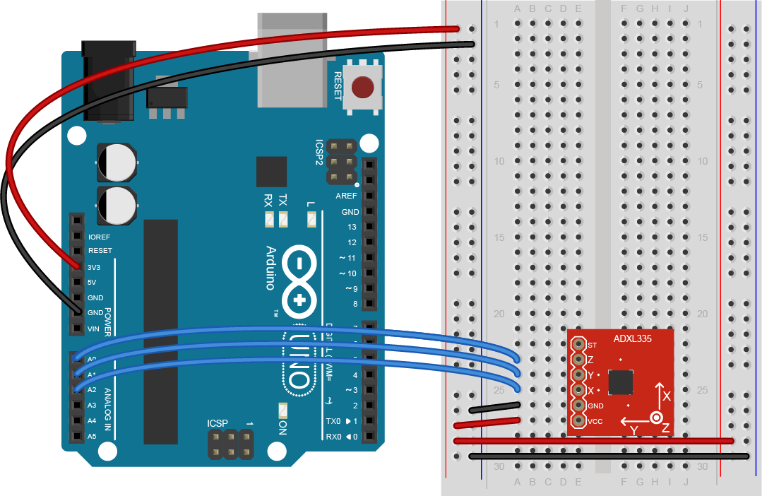
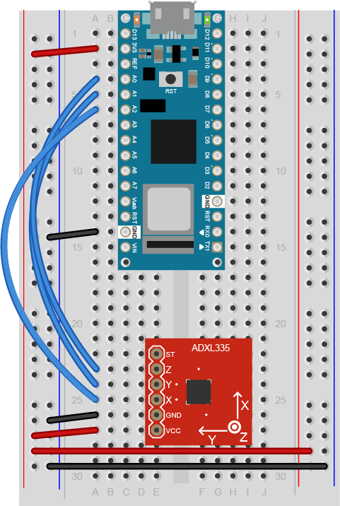
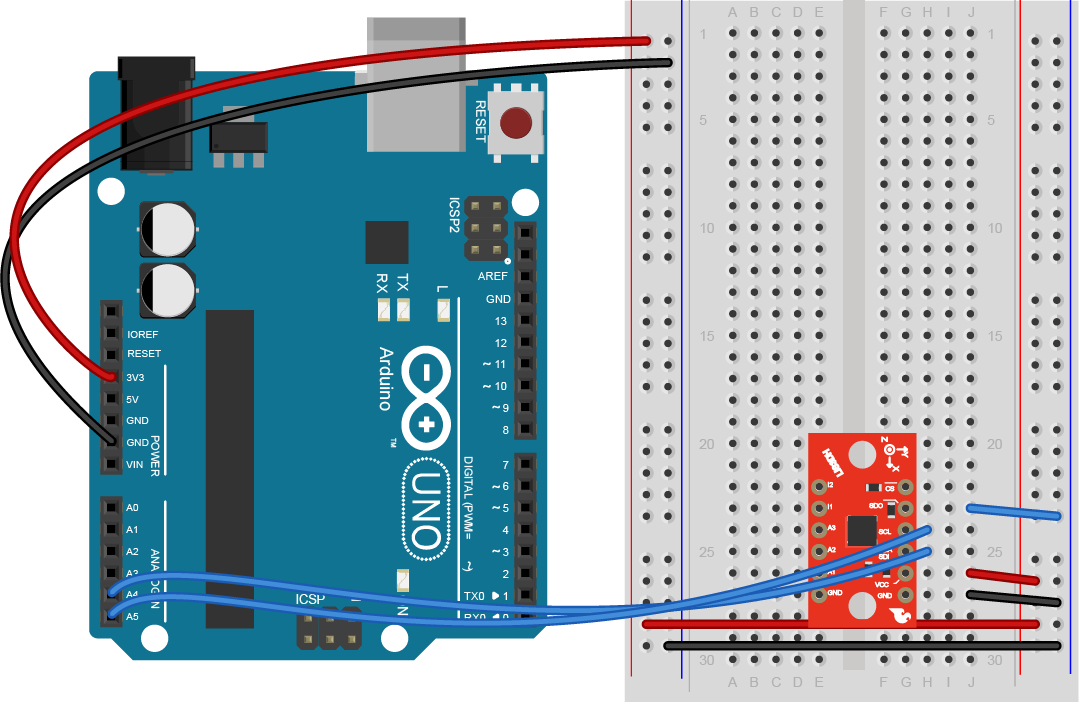
Figure 5 shows the schematic for connecting an ADXL335 to an Arduino, and Figures 6 and 7 show the breadboard view for the Uno and the Nano, respectively. For both boards, the accelerometer’s Vcc pin is connected to the voltage bus, and its ground pin is connected to the ground bus. The X axis pin is connected to the Uno’s analog in 2, the Y axis pin is connected to the Uno’s analog in 1, and the Z axis pin is connected to the Uno’s analog in 0.
Other analog IMUs are wired similarly.
Figure 5. Schematic view of an Arduino connected to an ADXL3xx accelerometer. The accelerometer’s Vcc pin is connected to 3.3V on the Arduino, and its ground pin is connected to ground . The X axis pin is connected to the Arduino’s analog in 2, the Y axis pin is connected to the Arduino’s analog in 1, and the Z axis pin is connected to the Arduino’s analog in 0.
Figure 6. Breadboard view of an Arduino Uno connected to an ADXL3xx accelerometer. The Uno is connected to a breadboard, with its 3.3V pin (not 5V as in other examples) connected to the voltage bus and its ground pin connected to the ground bus. The accelerometer is connected to six rows in the left center section of the breadboard beside the Uno.
Figure 7. Breadboard view of an Arduino Nano connected to an ADXL3xx accelerometer. The Nano is connected as usual, straddling the first fifteen rows of the breadboard with the USB connector facing up. Voltage (physical pin 2) is connected to the breadboard’s voltage bus, and ground (physical pin 14) is connected to the breadboard’s ground bus. The accelerometer is connected to six rows in the left center section of the board below the pushbutton.
The code below will read the accelerometer and print out the values of the three axes:
void setup() {
  Serial.begin(9600);
}

void loop() {
  int xAxis = analogRead(A2); // Xout pin of accelerometer
  Serial.print(xAxis);

  int yAxis = analogRead(A1); // Yout pin of accelerometer
  Serial.print(",");
  Serial.print(yAxis);

  int zAxis = analogRead(A0); // Zout pin of accelerometer
  Serial.print(",");
  Serial.println(zAxis);
}
Digital IMUs
Digital IMUs output a digital data stream via a serial interface, typically SPI or I2C. Unlike analog IMUs, these sensors can be configured digitally as well. Most support changing the sensitivity and the sampling rate, and some allow you to turn on and off features like tap detection or freefall detection.
Many digital IMUs are truly IMUs, in that they combine multiple sensors: accelerometer/gyrometer, accelerometer/gyrometer/magnetometer, and so forth.
Another advantage of digital IMUs is that they tend to convert their sensor readings at a higher level of resolution than a microcontroller’s analog input. While a microcontroller’s ADC is typically 10-bit (0-1023), many digital IMUs read their sensors into a 16-bit or even 32-bit result. This gives you greater sensitivity than an analog IMU.
Digital Accelerometer Example
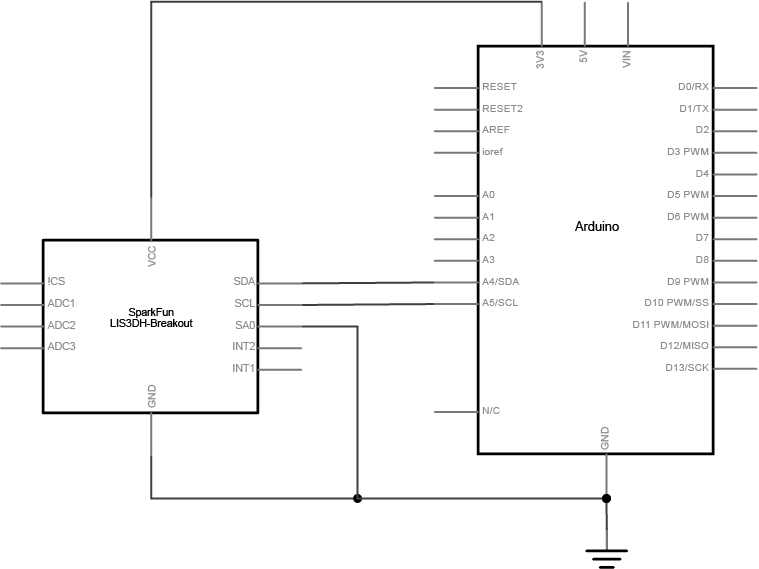
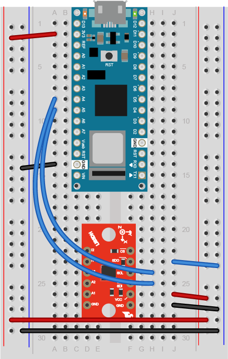
Figure 8 shows the schematic for connecting a LIS3DH accelerometer to an Arduino, and Figures 9 and 10 show the breadboard view for the Uno and the Nano, respectively. For both the Uno and the nano, the accelerometer’s Vcc pin is connected to the voltage bus, and its ground pin is connected to the ground bus. The SDA pin is connected to the microcontroller’s analog in 4, the SCL pin is connected to the microcontroller’s analog in 5 , and the SDO is connected to the ground bus. Other digital IMUs are wired similarly.
Figure 8. Schematic view of an Arduino connected to an LIS3DH accelerometer. The accelerometer’s Vcc pin is connected to 3.3V on the Arduino, and its ground pin is connected to the Arduino’s ground. The SDA pin is connected to the Uno’s analog in 4, the SCL pin is connected to the Uno’s analog in 5, and the SDO is connected to ground.
Figure 9. Breadboard view of an Arduino Uno connected to an LIS3DH accelerometer. The Uno is connected to a breadboard, with its 3.3V pin (not 5V as in other examples) connected to the voltage bus and its ground pin connected to the ground bus. The accelerometer is straddling the center of the board.
Figure 10. Breadboard view of an Arduino Nano connected to an LIS3DH accelerometer. The Nano is connected as usual, straddling the first fifteen rows of the breadboard with the USB connector facing up. Voltage (physical pin 2) is connected to the breadboard’s voltage bus, and ground (physical pin 14) is connected to the breadboard’s ground bus. The accelerometer is straddling the center of the board below the Nano.
The following code will read the accelerometer and print out the acceleration on each axis in g’s. This accelerometer has a 14-bit range of sensitivity. The code below configures the accelerometer for a 2g range, and converts the 14-bit range to -2 to 2g. This is a simplification of one of the LIS3DH library examples by Kevin Townsend. It uses Adafruit’s LIS3DH library, but will work for any breakout board for the LIS3DH. It’s been tested with both Sparkfun’s and Adafruit’s boards for this sensor:
#include "Wire.h"
#include "Adafruit_LIS3DH.h"

Adafruit_LIS3DH accelerometer = Adafruit_LIS3DH();

void setup() {
  Serial.begin(9600);
  while (!Serial);
  if (! accelerometer.begin(0x18)) {
    Serial.println("Couldn't start accelerometer. Check wiring.");
    while (true);     // stop here and do nothing
  }
  accelerometer.setRange(LIS3DH_RANGE_8_G);   // 2, 4, 8 or 16 G
}

void loop() {
  accelerometer.read();      // get X, Y, and Z data
  // Then print out the raw data
  Serial.print(convertReading(accelerometer.x));
  Serial.print(",");
  Serial.print(convertReading(accelerometer.y));
  Serial.print(",");
  Serial.println(convertReading(accelerometer.z));
}

// convert reading to a floating point number in G's:
float convertReading(int reading) {
  float divisor = 2 <<; (13 - accelerometer.getRange());
  float result = (float)reading / divisor;
  return result;
}
Here’s a link to some more examples for the LIS3DH which work with either Adafruit’s or Sparkfun’s LIS3DH board.
Built-in IMUs
Some microcontroller boards, like the Nano 33 IoT and Nano 33 BLE sense and the 101, have built-in IMUs. These are digital IMUs, and they’re connected to either the SPI or I2C bus of the microcontroller. This means you might have conflicts if you’re using them along with an external I2C or SPI sensor. For example, when you’re using them as an I2C sensor, you need to know their I2C address so you don’t try to use another I2C sensor with the same address.
Most built-in IMUs will come with a board-specific library, like the 101’s CurieBLE or the Nano 33 IoT’s Arduino_LSM6DS3 library. Otherwise, they will be identical to the digital IMUs, so even with a built-in accelerometer, you can get more information from the accelerometer’s datasheet or the library’s header files.
Nano 33 IoT Built-In IMU Example
The LSM6DS3 IMU that’s on the Nano 33 IoT is an accelerometer/gyrometer combination. You can get both acceleration and rotation from it. The IMU is built into the board, so there is no additional circuit.
The code example below will read the accelerometer in g’s and the gyrometer in degrees per second and print them both out:
#include "Arduino_LSM6DS3.h"

void setup() {
  Serial.begin(9600);
  // start the IMU:
  if (!IMU.begin()) {
    Serial.println("Failed to initialize IMU");
    // stop here if you can't access the IMU:
    while (true);
  }
}

void loop() {
  // values for acceleration and rotation:
  float xAcc, yAcc, zAcc;
  float xGyro, yGyro, zGyro;

  // if both accelerometer and gyrometer are ready to be read:
  if (IMU.accelerationAvailable() &&
      IMU.gyroscopeAvailable()) {
    // read accelerometer and gyrometer:
    IMU.readAcceleration(xAcc, yAcc, zAcc);

    // print the results:
    IMU.readGyroscope(xGyro, yGyro, zGyro);
    Serial.print(xAcc);
    Serial.print(",");
    Serial.print(yAcc);
    Serial.print(",");
    Serial.print(zAcc);
    Serial.print(",");
    Serial.print(xGyro);
    Serial.print(",");
    Serial.print(yGyro);
    Serial.print(",");
    Serial.println(zGyro);
  }
}
What To Look For in an IMU Library
Different vendors will generally write their own libraries for the IMUs they sell. When you’re looking at a given vendor’s product, take a look at the properties of the sensor in the vendor’s datasheet, and the list of public functions in the library’s API. Does the library give you the functions of the sensor that you need? If the sensor supports multiple sensing ranges, does the library give you access to setting and getting the range? Is it well-documented, and well-commented? Are there simple, clear, well-commented examples?
For example, both Sparkfun and Adafruit make breakout boards for the LIS3SH accelerometer. This accelerometer is typical for a digital accelerometer; it’s got I2C and SPI interfaces, operates at 3.3V, and has a range of acceleration sensitivity, from 2g to 16g. The Adafruit getting started guide and the Sparkfun getting started guide get you up and running, but neither provides a summary of all the functions in their libraries. To see that, you need to look at the header files for each library. Adafruit’s header file is exhaustively commented, which can take time to get through. The key public functions start around line 344. It relies on their Unified Sensor library, which adds some complexity, but there are some nice additions, like the click functionality that the accelerometer supports. Sparkfun’s header file is less thoroughly commented, but shorter. The key public functions start about line 116. If you only need the basic acceleration functions, it’s easier to use because of less dependency on other libraries. Both are good libraries, though, and you should choose based on the features you want and how easy you find each to use.
You could use either library with either breakout board, but there is one catch: when you’re using the board’s I2C synchronous serial interface, you have to pay attention to the address you use in the the Adafruit board defaults to a different I2C address than the Sparkfun one. SparkFun defaults to 0x19, while Adafruit defaults to 0x18. In I2C mode, the SDO pin switches the I2C default address between 0x18 and 0x19. Taking this pin HIGH sets the address to 0x19, while taking it LOW sets it to 0x18, so by changing this pin, you can choose which library you prefer. Both libraries also have the ability to change the address they use for the accelerometer as well.
Determining Orientation
Determining orientation from an IMU takes some advanced math. Fortunately, there are a few algorithms for doing it. In 2010, Sebastian Madgwick developed and published a more efficient set of algorithms for determining yaw, pitch, and roll using the data from IMU sensors. Helena Bisby converted Madgwick’s algorithms into a Madgwick library for Arduino, improved upon by Paul Stoffregen and members of the Arduino staff. Though it was originally written for the Arduino 101, it can work with any IMU as long as you know the IMU’s sample rate and sensitivity ranges. Here’s an example that uses the Madgwick library and the Nano 33 IoT’s LSM6DS3 IMU to determine heading, pitch, and roll:
#include "Arduino_LSM6DS3.h"
#include "MadgwickAHRS.h"

// initialize a Madgwick filter:
Madgwick filter;
// sensor's sample rate is fixed at 104 Hz:
const float sensorRate = 104.00;

void setup() {
  Serial.begin(9600);
  // attempt to start the IMU:
  if (!IMU.begin()) {
    Serial.println("Failed to initialize IMU");
    // stop here if you can't access the IMU:
    while (true);
  }
  // start the filter to run at the sample rate:
  filter.begin(sensorRate);
}

void loop() {
  // values for acceleration and rotation:
  float xAcc, yAcc, zAcc;
  float xGyro, yGyro, zGyro;

  // values for orientation:
  float roll, pitch, heading;
  // check if the IMU is ready to read:
  if (IMU.accelerationAvailable() &&
      IMU.gyroscopeAvailable()) {
    // read accelerometer &and gyrometer:
    IMU.readAcceleration(xAcc, yAcc, zAcc);
    IMU.readGyroscope(xGyro, yGyro, zGyro);

    // update the filter, which computes orientation:
    filter.updateIMU(xGyro, yGyro, zGyro, xAcc, yAcc, zAcc);

    // print the heading, pitch and roll
    roll = filter.getRoll();
    pitch = filter.getPitch();
    heading = filter.getYaw();
    Serial.print("Orientation: ");
    Serial.print(heading);
    Serial.print(" ");
    Serial.print(pitch);
    Serial.print(" ");
    Serial.println(roll);
  }
}
Conclusion
There are dozens of accelerometers, gyrometers, and IMUs on the market, and as they become more ubiquitous in electronic devices, they continue to get smaller, cheaper, and more power-efficient. The principles laid out here should give you a basis for getting to know new ones as needed.
We use a few different microcontroller boards in this class over the years, but for each one, there is a standard way we lay out the breadboard. This page details those layouts. In any lab exercise, you can assume the microcontroller and breadboard are laid out in this way, depending on the controller you are using. Figures 1, 2, and 3 show the layouts of an Arduino Nano 33 IoT, an Arduino Uno, an Arduino MKR.
Nano Layout
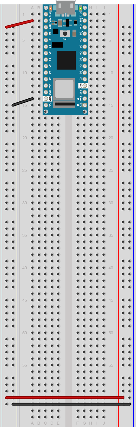
Figure 1. Breadboard view of an Arduino Nano on a breadboard
Figure 1. An Arduino Nano mounted on a solderless breadboard. The Nano is mounted at the top of the breadboard, straddling the center divide, with its USB connector facing up. The top pins of the Nano are in row 1 of the breadboard.
The Nano, like all Dual-Inline Package (DIP) modules, has its physical pins numbered in a U shape, from top left to bottom left, to bottom right to top right. The Nano’s 3.3V pin (physical pin 2) is connected to the left side red column of the breadboard. The Nano’s GND pin (physical pin 14) is connected to the left side black column.
These columns on the side of a breadboard are commonly called the buses. The red line is the voltage bus, and the black or blue line is the ground bus. The blue columns (ground buses) are connected together at the bottom of the breadboard with a black wire. The red columns (voltage buses) are connected together at the bottom of the breadboard with a red wire.
Uno Layout
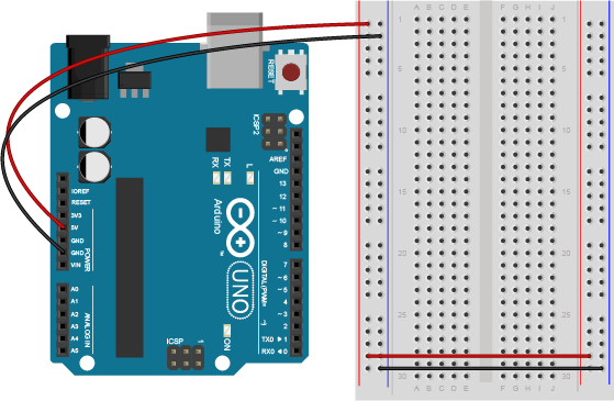
Figure 2. Breadboard drawing of an Arduino Uno on the left connected to a solderless breadboard on the right
Figure 2. An Arduino Uno on the left connected to a solderless breadboard, right. The Uno’s 5V output hole is connected to the red column of holes on the far left side of the breadboard. The Uno’s ground hole is connected to the blue column on the left of the board. The red and blue columns on the left of the breadboard are connected to the red and blue columns on the right side of the breadboard with red and black wires, respectively. These columns on the side of a breadboard are commonly called the buses. The red line is the voltage bus, and the black or blue line is the ground bus.
MKR Layout
Figure 3. Breadboard view of an Arduino MKR series microcontroller mounted on a breadboard
Figure 3. An Arduino MKR series board mounted on a solderless breadboard. The MKR is mounted at the top of the breadboard, straddling the center divide, with its USB connector facing up. The top pins of the MKR are in row 1 of the breadboard.
The Nano, like all Dual-Inline Package (DIP) modules, has its physical pins numbered in a U shape, from top left to bottom left, to bottom right to top right. The MKR’s Vcc pin (physical pin 26) is connnected to the right side red column of the breadboard. The MKR’s GND pin (physical pin 25) is connected to the right side black column. These columns on the side of a breadboard are commonly called the buses. The red line is the voltage bus, and the black or blue line is the ground bus.
The blue columns (ground buses) are connected together at the bottom of the breadboard with a black wire. The red columns (voltage buses) are connected together at the bottom of the breadboard with a red wire.
There are many text-only programming editors on the market, designed to be used with different programming environments. When you program using many different environments, it can be helpful to have one editor that you use for all of them, so your editing interface is consistent.
Organizing Projects
Most programming editors organize files in workspaces. A workspace is basically a folder with all your project’s files in it. So to get started, either open a folder or create a new folder, then make new files in it. For example, if you have an Arduino sketch called mySketch, it consists of a folder called mySketch and a file in it called mySketch.ino. A p5.js project is usually a folder called myProject with a few files in it: sketch.js, index.js, and the p5.js libraries.
Extensions or Plugins
Programming editors usually include a way to add extensions or plugins so that you can automate common tasks, use different programming languages easily, and so forth. For example, Visual Studio Code includes two useful plugins for physical computing, the Arduino plugin, which lets you compile Arduino projects and the Live Share plugin, which lets you share code live across a network.
Visual Studio Code
Microsoft Visual Studio Code is an open source programming editor from Microsoft that’s good for many toolchains at ITP: Arduino, p5.js, node.js, Python, and more. It’s designed for keyboard-only use, through the command palette, which can execute any command in the application using keyboard alone.
There are a few main areas of the VS Code application: the editor area, the file explorer, the consoles.
The explorer (command-shift-e) is where you look for files and folders within your workspace. There’s also a tab in the explorer called Outline where you can see a list of the functions in the open code window.
The editor (command-1, 2, 3, etc) is where you edit code. There can be multiple editors open in the same workspace, if you choose to do so.
The panel (control-`) are where you see the output console, the problems console, the command line terminal, serial terminals, and the debug console.
The command palette (command-shift-P) can execute any command in the application using keyboard alone. You can filter it by starting to type the name of the command you want. The Escape key dismisses the command palette.
Note that everything in VS Code is a file or a directory. Even the application Preferences are stored in a giant JSON file, and when you open preferences from the command palette, you can see this JSON file, or an abstracted HTML-style representation of it.
Keyboard Shortcuts
There are many keyboard shortcuts in VS Code, because it’s designed to be used without a mouse. If you can’t remember them all, there is a guide in the program. Type command-K-S to open it in the editor.
Shortcuts in command palette
Backspace, then type file name – will open any file in workspace
Colon, then type number – goes to line number in current editor window
> then type command. This is the default when you open the command palette. When you type any word, it will filter the command list to find matching commands. Then use up and down arrows to navigate the filtered list.
Getting to Files
Command-shift E shifts focus to the File explorer. The up and down arrows will move through the file names VoiceOver will read out the names. Once you know the file names, use either the file palette (command-P) or the command line terminal (described below) to open the file.
Command-P opens the File palette This is a variation on the command palette that opens files. It operates like the command palette. Type the filename to filter the available files in your current workspace.
Shortcuts in the Editor
To get to any line in the editor, open the command palette (command-shift-P), then backspace and type colon-line number to jump to any line. If you’re already in the editor, control-G-line number will do the same thing.
Working in the Panel
The Panel area contains the command line Terminal, the Output Console, the Problems Console, and the Debug Console.
Type control ` to open the terminal. This gets you to a terminal with your operating system’s command line interface in it. Here you can do all the things you can normally do on the command line: list files (ls), change directories (cd), and so forth. From the terminal,, you can also type “code <filename>” to open any file in the current directory into the editor.
Note that Control-G doesn’t jump you to a line number when you are in the terminal. Type control ` to close the terminal first.
Type control-shift-U to get to the Output console. This is where you’ll read the output of any commands run by a compiler, for example the Arduino compiler.
Extensions
Visual Studio Code lets you extend the application with additional modules downloaded from their online repository. Type control-shift-X to enter the Extensions browser. The Extensions browser works like the command palette: type a word to filter the list then use the up and down arrows to navigate the list.
Two useful plugins for physical computing are the the Arduino plugin by Microsoft and the Live Share plugin. If you have the Arduino IDE installed on your machine, the Arduino Plugin for VS Code lets you compile and upload for all the boards you have installed.The VS Live Share Plugin allows you to share code live with other users over a network in real time. Live share takes a few steps to get it set up, including a couple of trips to the browser to enable access through your GitHub account. The details are explained in the details page for the extension. Once it’s working, it’s a handy tool for sharing code live.
A Note on Notifications
Some actions or extensions pop up notification alerts over your application. These are called toasts in UX parlance, for reasons only the Secret UX Masters of the Universe understand. You can view all current notifications from the command palette: command-shift-P, then type notifications show. You can scroll through them with arrow keys when they are open. To dismiss them, command-shift-P, then type Notifications clear.
For users who prefer to use their own text editor, there is a command line interface version of the Arduino. “arduino-cli is an all-in-one solution that provides builder, boards/library manager, uploader, discovery and many other tools needed to use any Arduino compatible board and platforms.” It allows you to work with your favorite text editor, and to program in a text-only mode. The gitHub repository for the project includes a pretty good getting started guide to the arduino-cli on the main page, but there are a few extra steps you may want to take to set things up for more convenience. These instructions are written for MacOS, but should work on any POSIX operating system, and might work on Windows with the Linux Subsystem for Windows or with Cygwin, an older collection of Linux command line tools for Windows
Note that as of Sept. 2018, the arduino-cli is still in alpha, meaning that features are still subject to change.
Download the Application
From the gitHub repository, download the latest stable release of arduino-cli. Unzip the resulting download and move the unzipped application to your Applications directory (Linux users may prefer to move it to /usr/bin or /usr/local/bin). Then open the Terminal app (MacOS) or a shell window (Linux) to set things up.
Configure Your Command Line Environment
For those new to command line interfaces, there are a few terms that are helpful to know as well. The command line interface for MacOS is called a shell, specifically the bash shell.There are other shell environments for Linux and Unix (sometimes you’ll hear these collectively referred to as POSIX systems; here’s a longer introduction to command line interfaces in POSIX systems), but the bash shell is one of the most common. The parameters of the shell are called environment variables, and for the bash shell on MacOS, they are stored in a file called .bash_profile. They’re different for each user, so the .bash_profile file is kept in each user’s home directory. The path to this directory is /Users/username on MacOS, or /home/username on Linux. The shortcut for the home directory is ~. For example, ~Documents/ is the path to your Documents folder. When you’re on the command line, you can always get back to the home directory by typing cd and then pressing enter. You can check what directory you are in by typing pwd (for print working directory)
It’s helpful to add a few modifications to your command line environment to make arduino-cli easier to work with. First, open .bash_profile in your favorite text editor. The dot at the beginning of the filename means this is hidden file, so it won’t show up when you list files. To see it using the command line list command (ls), type ls -a and you’ll see all the hidden files. To open any file in your text editor, type
open -a editorName filename
Replace editorName with the name of your editor, For example, to open the .bash profile in XCode, type open -a editorName .bash_profile.
That open trick is so useful that you’ll want to add a shortcut to your profile. At the end of the file, add the following line:
alias xcode="open -a xcode"
Change the alias name and the editor name as you see fit. Now you can open your editor from the command line. This is useful for other development activities, like working in node.js, p5.js, or Python. Next you need to add the Applications directory to your PATH environment variable so that the shell knows where to find it. Add a new line to the file as follows:
export PATH=${PATH}:/Applications
Arduino-cli does not include the built-in examples that come with the original Arduino graphic IDE. If you’ve installed the original IDE, you have them, but you might want to create an shortcut in your Arduino sketches directory to get to them. Here are the paths to the examples for MacOS, Windows, and Linux:
MacOS: (assuming you installed the Arduino IDE in your applications folder already): /Applications/Arduino.app/Contents/Java/examples
Windows 10: C:\Users\”USERNAME”\AppData\Local\Arduino15\packages\arduino
Linux: ~arduino-1.8.x/examples
To create the shortcut, change directories to your sketch directory and type:
and you’ll then have be able to get to them directly from the sketches directory. On Linux or Windows, change the path accordingly.
Finally, if you find the default shell prompt too long, you can add a custom shell prompt. For example, the default MacOS shell prompt is computer-name:directory username$. This appears after you run every process on the command line, before you get to run a new process. To shorten the command prompt to a single $, add this line to your .bash profile:
export PS1="$ "
The $ prompt is common enough that you’ll usually see it at the beginning of any command line instructions in tutorials. If you see it, type what follows it at your command prompt.
To put these changes into effect, save your .bash_profile file, type exit on the command line to close your command line session, then re-open a new shell window. In the new window, you should see that the command prompt is now just a $ symbol. To test your editor shortcut, type
$ touch foo.txt
This will create a new file called foo.txt in your current directory. Then type
$ xcode foo.txt
This should launch XCode (or whatever editor you chose) and open the file foo.txt.
Using arduino-cli
To use arduino-cli on the command line, type its name followed by whatever parameters you want to use. If you type arduino-cli with no parameters, you’ll get a list of the commands available. The application that you downloaded is probably not just called arduino-cli, however. It’s probably something longer, like arduino-cli-0.2.2-alpha.preview-osx. Fortunately, you don’t have to type the whole name. The shell will auto-complete any command you type if it can when you press the tab key. If you type ard then press tab, it should autocomplete the name of the program. In this tutorial, the application name will be shortened to arduino-cli.
To create a new sketch, type:
$ arduino-cli sketch new SketchName
This will create a new sketch in the default Arduino sketch directory. On MacOS, this directory is ~Documents/Arduino/, so the sketch would be in ~Documents/Arduino/. To get to the directory to work on this new sketch, type:
$ cd ~Documents/Arduino/SketchName
Now that you’ve got your command line environment set up, the getting started with arduino-cli guide will take you through the steps of creating a new sketch, configuring the environment, and uploading it. Below is a summary of the commands you’ll use the most.
New Sketch:arduino-cli sketch new mySketch – creates a new sketch called mySketch in the default Arduino sketch directory
List Available boards:arduino-cli board list – list all boards attached to the computer. This is equivalent to getting the port list in the Arduino graphic IDE.
List All Known Boards:arduino-cli board listall – list all boards in your boards manager. This is equivalent to getting the boards list in the graphic IDE. This produces a long list, so if you wanted to search it for a particular subset, you might use the POSIX grep command like so:
$ arduino-cli board listall | grep mkr
The preceding command would list all known boards with the substring mkr in their name.
Compile:arduino-cli compile -b board:name path/to/sketch – compile the sketch for the given board name. This is equivalent to the Verify command in the graphic IDE. You don’t need the sketch path if you’re already in the sketch directory. For example, to compile the sketch in the current directory for the Uno:
$ arduino-cli compile -b arduino:avr:uno
Or for the MKRZero:
$ arduino-cli compile -b arduino:samd:mkrzero
Attach Board:arduino-cli board attach board:name – attaches a specific board name to a sketch. This is equivalent to choosing a board in the graphic IDE. If you do this when you first set up a new sketch, you won’t need to give a board name every time every time you compile, you can just type
$ arduino-cli compile
Upload:arduino-cli upload -p portname – upload compiled sketch to the portname given. This is equivalent to uploading in the IDE. Note that this command does not re-compile before uploading. For example:
$ arduino-cli upload -p /dev/cu.usbmodem1411
Find a core:arduino-cli core search coreName – searches for known processor architectures. You can search by processor type, like AVR or M0, or you can search by board name, like Mega or MKR. For example:
$ arduino-cli core search mkr
Install a core:arduino-cli core install coreName – installs a core once you find it. ou must use the full core name, though. For example the core search for MKR above resulted in a core called arduino:samd. To install it, type:
$ arduino-cli core install arduino:samd
Find a library:arduino-cli lib search libraryName – searches the Arduino library manager index for libraries containing the word libraryName. For example, the following will list all MQTT-related libraries in the index:
$arduino-cli lib search mqtt
Install a library: arduino-cli lib install libraryName – install a library that’s listed in the Arduino library manager index. For example:
$ arduino-cli lib install WiFiNINA
or for libraries with multiple word names, use double quotes around the name like so:
$ arduino-cli lib install "Arduino Low Power"
For more information, see the arduino-cli guide. Check back frequently for changing features until it is out of alpha.
Using the Serial Port
On MacOS and Linux, the command line allows you to read input from a serial port just as you would from a file, using the cat command. cat /dev/cu.usbmodemXXXX will open an Arduino’s serial port, if no other application has it open already. control-C will close it.
This page explains the basic pin functions that most microcontrollers share, and offers some tips for switching from one microcontroller to another. Since the tutorials on this site are all written with the Arduino Uno in mind, and students may be using other controllers, you may need to know how to “convert” a tutorial from the controller it’s written for to your own controller. In order to get the most out of it, you should know something about electrical circuits, and what a microcontroller is and what it can do. This video might help: Hardware functions in a microcontroller
What Do All These Pins Do?
A typical microcontroller can have between 6 and 60 pins on it, to which you’re expected to attach power connections, input and output connections, and communications connections. Every microcontroller has different configurations for its pins, and often one pin will have more than one function. This combining of functions on one pin is called pin multiplexing.
Every microcontroller has names for the pins specific to its hardware, but the Arduino application programming interface (API) provides a set of names for pins and their functions that should work across all microcontrollers that are programmable with the API. So, for example, A0 will always be the analog input pin 0, whether you’re on an Uno, 101, MKRZero, MKR1000, or other Arduino-compatible board. When you connect to the pin with the same function on another board, your code should operate the same, even though the physical layout of pins is different.
Every board has an operating voltage that affects its pins as well. The operating voltage, which is the same as the voltage of the GPIO pins, is labeled below. If you’re connecting a component to a board with a lower voltage than the component, you’ll need to do some level shifting.
Pin Diagrams
Microcontrollers typically come in a variety of physical forms, or packages. Sparkfun has a nice tutorial on integrated circuit package types if you want to know more. Pin numbering on any integrated circuit, including microcontrollers, starts at top left corner, which is usually marked with a dot. From there, you count around the chip counter-clockwise. For modules like the Arduino Uno, this numbering doesn’t hold up, since the board has several pin headers. The pin headers are usually numbered, and the pins of each header are counted. Unfortunately, header numbering does not always follow the same patterns as IC numbering.
Microcontroller pins are referred to by their physical pin (where they are physically on the board) and their functional pin names (what they do). For example, the Arduino Nano’s physical pin 20 is digital I/O pin 2.
Arduino Nano Series
Arduino Nano 33 IoT Pin diagram
The Arduino Nano boards, like the Nano Every, Nano 33 IoT, Nano 33 BLE, Nano 33 BLE Sense, and Nano RP2040 Connect have a number of similar features. The Nano 33 IoT is shown in Figure 1, but the other Nanos have the same pin layout. The pin numbering follows the U-shaped pattern of a typical integrated circuit as described above; pin 1 is on the top left, and pin 30 is on the top right. The pins, summarized, are as follows:
Physical pin 1: Digital I/O 13
Physical pin 2: 3.3V output
Physical pin 3: Analog Reference
Physical pin 4-11: Analog in A0-A7; Digital I/O 14-21
Physical pin 12: VUSB (not normally connected)
Physical pin 13: Reset
Physical pin 14: Ground
Physical pin 15:Vin
Physical pin 16: Digital I/O pin 1; Serial1 UART TX
Physical pin 17: Digital I/O pin 0; Serial1 UART RX
Physical pin 18: Reset
Physical pin 19: Ground
Physical pin 20-30: Digital I/O pins 2-12
PWM Pins: on the Nano 33 IoT, the following pins can be used as PWM pins: digital pins 2, 3, 5, 6, 9, 10, 11, 12, A2, A3, and A5. One pin A0, can also be used as a true analog out, because it has a digital-to-analog converter (DAC) attached. On the Nano Every, only pins 3, 5, 6, 9, and 10 can be used as PWM pins. On the Nano 33 BLE, all digital pins can be used as PWM pins.
SPI Pins:
SDI- digital pin 12 (physical pin 30)
SDO – digital pin 11 (physical pin 29)
SCK – digital pin 13 (physical pin 1)
CS – digital pin 10 (physical pin 28)
I2C Pins:
SDA – pin A4 (physical pin 8)
SCL – pin A5 (physical pin 9)
UART Pins:
Serial 1 TX: digital pin 1 (physical pin 16)
Serial1 RX: digital pin 0 (physical pin 17)
Notes on the Nano Series
The Nano Every operates on 5V. The Nano 33 IoT, 33 BLE, and RP2040 Connect operate on 3.3V.
The Nano 33 IoT is based on the SAMD21 processor, just like the MKR boards. It has a NINA W102 radio that can communicate using Bluetooth 4.0 or WiFi, just like the MKR 1010. The RP2040 Connect has the same radio. It also has a real-time clock and an IMU sensor. For more on this board, see the Introduction to the Nano 33 IoT.
The Nano 33 BLE is based on the nRF 52840 microcontroller. It can communicate using Bluetooth 5.0
The Nano Every is based on the ATMega4809 microcontroller. It is functionally most similar to the Uno’s Atmega328 processor.
The Nano RP2040 Connect is based on the Raspberry Pi RP2040 processor, a dual SAMD21 processor.
On the Nano Every, pins 16 and 17 (TX and RX) are the serial port called Serial; they are also attached to the USB-Serial microcontroller on board. On the 33 IoT and 33 BLE, they are the serial port called Serial1 and are not attached to the USB serial port.
On the Nano 33 IoT as opposed to other Arduino Nano boards, pins A4 and A5 have an internal pull-up resistor and default to the I2C functions.
On the Nano 33 IoT and Nano 33 BLE, the VUSB pin does NOT supply voltage but is connected through a jumper, to the USB power input. You need to solder the jumper on the bottom of the board to use VUSB.
Interrupts: All the Nano 33 IoT’s, Nano 33 BLE’s, and Nano Every’s digital pins can be used as hardware interrupts. However, some repeat, so check the AttachInterrupt guide for the best pins to use as interrupts.
Arduino Uno Rev 3
Arduino Uno Rev 3 Pin diagram
The Arduino Uno Rev 3, shown in Figure 1, is the classic Arduino model. The pin numbering follows the U-shaped pattern of a typical integrated circuit as described above; pin 1 is on the top left, and pin 30 is on the top right. The pins, summarized, are as follows:
Physical pin 1: not connected
Physical pin 2: I/O reference voltage
Physical pin 3: Reset
Physical pin 4: 3.3V output
Physical pin 5: 5V output
Physical pin 6-7: Ground
Physical pin 8: Vin
Physical pin 9-14: Analog in A0-A5; Digital I/O 14-19
Physical pin 15-28: Digital I/O pin 0-13
Physical pin 29: Ground
Physical pin 30:Analog Reference
Physical pin 31: I2C SDA; Digital I/O pin 18; Analog in A4
Physical pin 32: I2C SCL; Digital I/O pin 19; Analog in A5
PWM Pins: on the Uno Rev 3, the following pins can be used as PWM pins: digital pins 3, 5, 6, 9, 10, 11.
SPI Pins:
SDI- digital pin 12 (physical pin 27; digital I/O pin 12)
SDO – digital pin 11 (physical pin 26; digital I/O pin 11)
SCK – digital pin 13 (physical pin 28; digital I/O pin 13)
CS – digital pin 10 (physical pin 25; digital I/O pin 10)
I2C Pins:
SDA – pin A4 (physical pin 13 or 31; Analog in pin A4)
SCL – pin A5 (physical pin 14 or 32; Analog in pin A5)
UART Pins:
Serial TX: digital pin 1 (physical pin 16)
Serial RX: digital pin 0 (physical pin 15)
Notes on the Uno Rev 3
At the bottom center of the Uno board is a six-pin connector called the In-Circuit Serial Programming connector (ICSP). It has two rows of pins, labeled as follows:
Top row (left to right): Reset, SCK, SDI
Bottom row (left to right): Ground, SDO, +5V
On the top right of the Uno is another six-pin connector. The Uno has a second microcontroller on board to handle USB-to-serial communications. This is the ICSP header for that microcontroller.
The Serial port called Serial is attached to pins 0 and 1, and to the USB-Serial micrcontroller on board.
Interrupts: on the Uno rev. 3, only digital pins 2 and 3 can be used as interrupts.
Arduino MKR Series
Mkr Zero Pin diagram
The Arduino MKR series are intended for advanced RF applications. They have the same SAMD Cortex M0+ as the Nano 33 IoT, and a built-in rechargeable battery connector and charging circuit. Like most of the Nanos, the MKRs are 3.3V boards. There are several boards in the MKR line for different connectivity needs:
The pin numbering follows the U-shaped pattern of a typical integrated circuit as described above; pin 1 is on the top left, and pin 28 is on the top right. The pins, summarized, are as follows:
Physical pin 1: Analog Reference
Physical pin 2-8: Analog in A0-A6
Physical pin 9-14: Digital I/O pin 0-5
Physical pin 15-23: Digital I/O pin 6-14
Physical pin 24: Reset
Physical pin 25: Ground
Physical pin 26: 3.3V output
Physical pin 27: Vin
Physical pin 28: 5V output
PWM Pins: on the MKR series, the following pins can be used as PWM pins: digital pins 0 – 8, 10, 12, analog pins A3, A4.
SPI Pins:
SDI- digital pin 12 (physical pin 19; digital I/O pin 10)
SDO – digital pin 11 (physical pin 17; digital I/O pin 8)
SCK – digital pin 13 (physical pin 18; digital I/O pin 9)
CS – any other digital pin
I2C Pins:
SDA – Digital I/O pin 11 (physical pin 19)
SCL – Digital I/O pin 12 (physical pin 20 )
UART Pins:
Serial TX: digital pin 14 (physical pin 21)
Serial RX: digital pin 13 (physical pin 20)
Notes on the MKR Series
Serial: The MKR series boards have two hardware UARTs.The first one, UART0 (aka Serial in your sketches) is attached directly to the USB port not to any pins. GPIO pins 13 and 14 are Serial1
Battery in: LiPo, 3.7V, 700mAh min Recharging circuit on board.
Interrupts: On the MKR series, pins 0, 1, 4, 5, 6, 7, 8, 9, A1, and A2 can be used as interrupts.
Pin Functions Explained
In order to make sense of all of this, it helps to know the general functions of a microcontroller. There are a few common functions:
Power: Every microcontroller will have connections for power (often labeled Vcc, Vdd, or Vin) and ground. A bare microcontroller will have only those, but modules like the Arduino, the Raspberry Pi, and others also have voltage regulators and other components on board. On these, it’s common to see an unregulated voltage input (Vin) and a regulated voltage output (5V and 3.3V on the Uno, for example).
Clock: Every microcontroller needs a clock. The bare microcontroller chip usually has two pins for this. On a module, the clock is usually built onto the board, and the pins are not exposed.
General Purpose Input and Output (GPIO): Most pins on a microcontroller can operate as either a digital input or digital output.
Hardware Interrupts: Many microcontrollers have a subset of their GPIO pins attached to hardware interrupt circuits. A hardware interrupt can interrupt the flow of a program when a given pin changes its state, so you can read it immediately. Some higher level functions like asynchronous serial and PWM sometimes use these interrupts. They’re also good for very responsive reading of digital inputs.
Analog Input (ADC): Not all microcontrollers have an analog-to-digital converter (ADC), but those that do have a number of pins connected to it and act as inputs to the ADC. If there are analog inputs, include analog reference pin as well, that tells the microcontroller what the default high voltage of the ADC is.
Pulse Width Modulation (PWM): Few microcontrollers have a true analog voltage output (though the MKR1000 does), but most have a set of pins connected to an internal oscillator that can produce a pseudo-analog voltage using PWM. This is how the analogWrite() function in Arduino works.
Communications:
Universal Asynchronous Receiver/Transmitter (UART): Asynchronous serial communication is managed by a Universal Asynchronous Receiver/Transmitter, or UART, inside the processor. The UART pins are usually attached to internal hardware interrupts that can interrupt the program flow when new serial data arrives, so you never miss a byte. It’s possible to manage serial communication in software alone, but at high speeds, you’ll see more errors.
Synchronous Serial: SPI and I2C: Most microcontrollers also have dedicated modules in the processor to handle the two most common forms of synchronous serial communication.
The Serial-Peripheral Interface (SPI) bus has four dedicated pins: Serial Data Out (SDO), also called Controller In, Peripheral Out (CIPO); Serial Data In (SDI), or Controller Out, Peripheral In (COPI); Serial Clock (SCK) and Chip Select (CS). Many miccrocontrollers are programmed via SPI through an In-Circuit Serial Programming header (ICSP) as well.
The Inter-Integrated Circuit (I2C) bus has two pins: Serial Data (SDA) and Serial Clock (SCL).
Reset: All microcontrollers have a pin which resets the program. Usually you take this pin low to reset the controller.
IORef: this is the operating voltage of the board. The Uno and 101 have this pin so that shields can read this voltage to adjust their own output voltages as needed. Not all shields have this functionality.
With a wide variety of Arduino and Arduino-compatible options on the market, students often ask “which is the best controller for me to get?” What follows is a guide how to decide what to choose. This is by no means an exhaustive list, it only includes boards I use regularly enough to recommend.
The lab exercises for this class were originally written for the Arduino Uno. Currently we teach it with the Arduino Nano 33 IoT, for reasons explained below.
The things you should consider in picking a controller, other than price:
Is this controller compatible with my other components?
Does it operate on the same voltage range?
Does it have the correct interface (e.g. asynchronous serial, I2C, SPI)?
Is it programmable with the tools I am using and any existing code I am using?
What physical inputs and outputs do I need?
With what other devices does it need to communicate?
What protocols will they use (e.g. WiFi, Bluetooth, USB, etc)?
What aspects of the project can be handled by those other devices?
Is the form factor one I can work with?
The processor at the core of the Uno, Atmel’s ATMega328, is an 8-bit microcontroller. The ATMega328 is one of the few processors that still comes in a breadboard-friendly DIP package, so you can even build your own Uno-compatible circuit on a breadboard if you want to save money. In projects where you’re using multiple controllers, the DIY breadboard option is a smart choice. However, it’s not a task for you if you aren’t yet comfortable building circuits and reading schematics.
Nowadays, 32-bit microcontrollers are available for about the same price or cheaper than 8-bit controllers. The Arduino Nano series and MKR series are mostly 32-bit processors (the Nano Every is still 8-bit) that can do all that the original Uno can do and more. These newer controllers have more processing power and memory for your program than the Uno and other 8-bit controllers, and with the various connectivity options (WiFi, Bluetooth) that these boards offer, you’ve got more room to grow. If you’re buying your first controller, your best choice is probably one of the 32-bit controllers. The Nano line and the MKR line are the ones I currently use the most.
3.3V? 5V? What’s the difference?
1.7V, of course (a little electrical humor).
The Arduino Uno and the boards that came before it operated on 5 volts DC. However many newer controllers, including all the ones here, and the embedded Linux boards like the BeagleBone and the Raspberry Pi, operate on 3.3 volts instead. Many older components, like the Sharp IR rangers that are popular in physical computing, operate on 5 volts, and many newer ones operate on 3.3 volts. Because of this change, you often need to adjust the voltage output of one component before it goes into another component. This is called level shifting. It’s a common technique you learn how to deal with when you work with many different components.
I Need A Lot of Input and Output…
Many physical computing projects need lots of input and output connections to read lots of sensors. There are lots of strategies for handling this. Many of the most common strategies are described in chapter 14 of Physical Computing: Sensing and Controlling the Physical World by Dan O’Sullivan and Tom Igoe. Although that book describes processors other than the Arduino, the circuits and techniques described work well with Arduino-compatible boards.
If you just want a single board with a lot of pins, consider the Arduino Due. The Due has an Atmel SAM3X8E ARM Cortex-M3 processor, which is a more powerful version of the processor than the M0 in the MKR boards. This, or the strategies in Physical Computing, are probably the best option for multiple I/O for beginners.
If you’re feeling more advanced and want another approach, consider building your project with multiple processors. You can build your own Uno variant on a breadboard, or you can use the even smaller ATTiny84 and ATTiny85 controllers. These controllers have only a few I/O pins, but they are a couple of dollars each, and David Mellis has an excellent guide to programming them. You can link several of them together in one circuit and have each one control a handful of your I/O pins, then use one of the other processors mentioned here as a main controller.
Connectivity
Increasingly, projects need not just basic input and output, but also WiFi, Bluetooth, USB, or some other form of connectivity. This is where the more modern boards outshine the Uno and derivatives. Bluetooth, WiFi, and USB are pretty easy to get on a variety of boards. Other radio types are less common, but there’s a board for pretty much every form of connectivity.
Nano
The Nano family is a good, inexpensive starting place for beginners, with lots of room to grow. The Nano Every is thoroughly compatible with the Uno’s architecture for a lower price. It operates on 5 volts, just like the Uno. The Nano 33 IoTis a 3.3V board, with lots of extra features. It has the same processor as the MKR series, the SAMD21 Cortex M0+ ARM processor, and has a Bluetooth and WiFi radio on board, at a lower price than the MKR line. At the top of the line, the Nano 33 BLE and BLE Sense and the Nano RP2040 Connect have enough processor power to run TinyML machine learning models as well.
Code you’ve written for the Uno will also run on the Nanos as well, but you’ll need to pay attention to which pins your external components are connected to, since the layout is not the same as the Uno. All of the Nanos except the Every are 3.3V boards, meaning that the default voltage is 3.3 volts, not 5 volts. This can present some challenges when dealing with sensors that operate on 5 volts, though nowadays most sensors are 3.3-volt compatible.
MKR
The MKR family are handy when you need advanced connectivity features.They have the same SAMD Cortex M0+ as the Nano 33 IoT, and a built-in rechargeable battery connector and charging circuit. Like most of the Nanos, the MKRs are 3.3V boards. There are several boards in the MKR line for different connectivity needs: The MKRZero has a built-in MicroSD card. The MKR1000 and MKR1010 are WiFi boards; the MKR1010 has Bluetooth as well. The MKR1300 and MKR1310 have LoRa and LoRaWAN connectivuty. The MKR1400 has a GSM radio, and the MKR1500 has a NB IoT 3G radio. In addition, there are several special purpose shields for the MKR boards.
Caveat: be wary of cheap derivatives, clones, and counterfeits of these boards. There are a number of very good derivatives that offer extra features, or different layouts. There are also a number of derivatives and clones that try to look the same, but use lower quality components or spend less time on inspecting assembled boards. We see a few broken projects every year that are due to a clone board failing. Many of the vendors linked from this page sell their own Arduino-compatible variants that are reputable, if you want to look for derivatives.
Feather
Adafruit’s Feather M0 boards are also good DIP-format boards. They use the same processor, Atmel’s CortexM0+, they also use the DIP package, and they come in a variety of special-purpose variations. The basic Feather M0 Proto board has just the processor, it’s like a MKR1000 without the Wifi. The Feather Adalogger M0 is the same thing with a built-in SD card. The Feathers also have a built-in LiPo battery charger.
With one of the boards above, you can do everything covered in the labs for this class, with a faster and more capable processor than the Uno. Everything that follows is for readers who are already comfortable with microcontrollers, and looking for more info for advanced projects. For more information, see the comparison chart and vendors at the bottom of this page.
ESP
You could also consider Espressif’s processors, if you need lots of processors connected wirelessly. They’re not as inexpensive as the ATTiny processors, but they have built-in WiFi. Espressif’s ESP8266 processor is a very inexpensive 32-bit processor with WiFi built in. It’s very popular when you’re building projects that need lots of WiFi devices. THE ESP boards have relatively little I/O, however, and only one analog in that can only read a 1-volt range. So the lower cost is often lost in extra components to add I/O. The Feather Huzzah ESP8266 is a good implementation of the ESP8266, as is Spark Fun’s ESP8266 Thing Dev board. Many other vendors sell their own version of the ESP8266 board, but these are the two that I’ve used which are simplest for relative beginners to use. The ESP8266 WiFi libraries are based on the Arduino WiFi101 libraries, so code is relatively compatible with the MKR1000. The ESP32 is an upgraded version of the ESP8266.
The ESP8266 boards can also run other languages. There’s a port of JavaScript, a MicroPython version, and Lua version that are relatively mature, and others still in development. Watch the ESP repositories for updates.
The ESP8266 boards are not great for the absolute beginner, but they’re relatively easy for intermediate users, and handy when you need a lot of processors networked inexpensively.
Can I Program it in Python/JavaScript?
Yes, but there are limitations. There are microcontrollers on the market that you can program with scripting languages like Python and JavaScript. The Espruino is a good version of JavaScript for microcontrollers, and the MicroPython board does the same for Python. The BBC Micro:Bit runs both. The Espruino JavaScript engine is available for the ESP8266 as well. The RP2040 Connect and some of the Feathers run Python as well.
Although these scripting engines seem enticing for microcontroller use, they come at a cost. Scripting engines can never run your code as fast as compiled code, and sometimes the timing can be inconsistent, because the engine’s cleaning up memory and not listening to your I/O pins. Any good programming tool needs a good framework for building libraries as well. When you’re looking at new tools like this, check what libraries are available, and what the framework for building libraries looks like, and how many programmers are using it. Also consider that any scripting language on a microcontroller means that your source code, not the compiled binary program, is present on the processor itself. This is no big deal for hobbyists, but is a potential security risk for commercial products.
What About Embedded Linux?
There are a number of different embedded Linux processors on the market now that are in the same price range as microcontroller boards. The Raspberry Pi and the BeagleBone Green Wireless are excellent examples of this, and good products. These boards are getting more capable all the time. Many of the Processing and P5.js/node.js examples for this class run on the Raspberry Pi 2 and 3, for example, or the BeagleBone Green Wireless.
For this intro to physical computing class, they are overkill, however, because they require you to learn how an embedded operating system works in addition to the electronics, programming, and physical interaction design we’re already covering. It’s not uncommon to combine a microcontroller with an embedded linux processor, with the former handling physical I/O and the latter handling media control or network communication. The two communicate via asynchronous serial, just like your laptop and your microcontroller will do in the serial labs in this class.
For the purposes of this class, you’re welcome to explore the embedded Linux boards independently once you’ve shown mastery of the material covered in class. Your projects will be evaluated mostly on how well they demonstrate good physical interaction design, however.
Where To Get Boards
The Arduino boards mentioned here are carried by the Arduino online store as well as many of the vendors mentioned here: Adafruit, Spark Fun, Seeed Studio, and Digikey are the vendors I use most frequently. For Seeed Studio products in the US, Digikey is a useful reseller. It’s worth comparing them all for pricing, though the differences are not usually large.